
Recent years have witnessed a dramatic rise in neo-Nazi, white supremacist ‘fight clubs’. Typically, these clubs bear the relatively innocuous moniker of ‘Active Club’ (AC). Though originally an American phenomenon, initiated by Robert Rundo, originally from California, ACs have spread to Europe and beyond, establishing chapters, building networks, recruiting young men under the guise of fitness, combat sports, and ‘brotherhood’. This blog follows up on the valuable research done by the Global Project Against Hate and Extremism (GPAHE), which has tracked the diffusion of ACs (e.g., in a 2023 report). Specifically, it draws on the recent (late June 2025) release of updated GPAHE data on extant ACs. The PDF of tabular data is available below. A reworked version of the data, correcting some inaccuracies and adding approximate locations is available for download at the bottom of this page.
Active Clubs usually style themselves as male-oriented, fitness- and martial-arts organisations that more or less openly promote a white nationalist ideology. Rundo and co-originator Denis Kapustin, a Russian neo-Nazi, elaborated the idea of ACs as ‘white nationalism 3.0’, building on Louis Beam’s idea of leaderless resistance by aiming to create a network of sporting clubs that share symbols and ideological tenets. This pattern is similar to the model of groups like Blood & Honour, Hammerskins, and Identitarian groups.
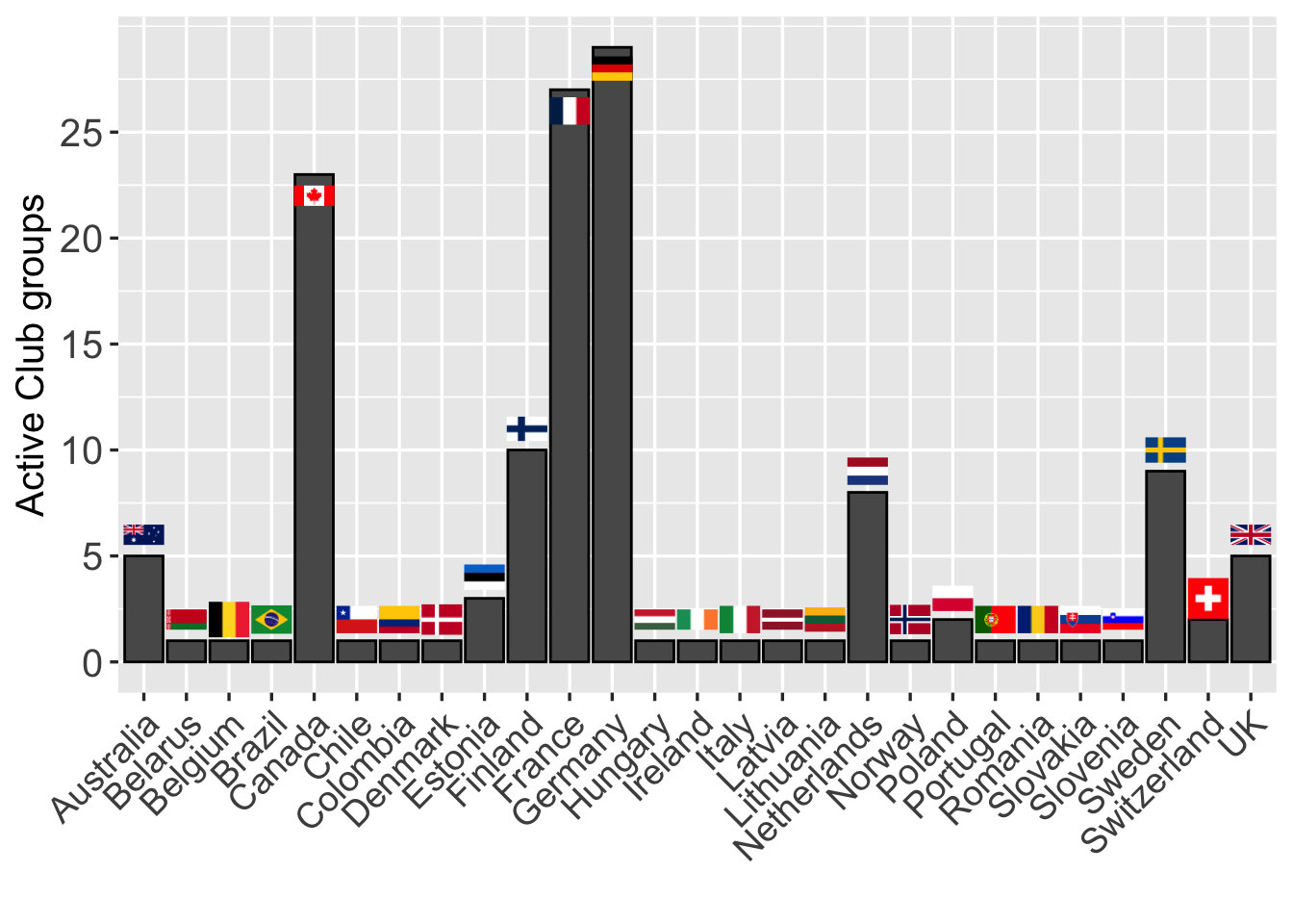
Active Clubs by country
The rapid spread of ACs is perhaps unique. According to the June 2025 update by GPAHE, there are ACs in at least 27 countries. This proliferation has developed in the space of only a few years. While the plurality of ACs are located in North America (especially the United States), chapters have emerged in many European countries. Often, ACs in Europe have been incorporated into preexisting right-wing extremist organisational structures, such as Der III. Weg (‘The Third Way’) in Germany, and are more centrally organised than in the United States.
The chart below (which excludes the United States and the upwards of 90 ACs based there) shows that in Europe France and Germany have the most ACs, followed by Finland, Sweden, and the Netherlands. But there is at least one AC in most European states.
Click to expand/collapse the code
ACs_country <- gpahe_ACs %>%
  filter(Country!="United States") %>%
  group_by(Country) %>%
  summarise(Groups = n())

flags_df <- ACs_country %>%
  distinct(Country) %>%
  mutate(
    iso2 = countrycode::countrycode(Country, origin = "country.name", destination = "iso2c")
  ) %>%
  mutate(
    # fix EU ISO2 and provide custom flag
    iso2 = ifelse(Country == "EU", "eu", iso2),
    flag_url = ifelse(
      Country == "EU",
      "https://upload.wikimedia.org/wikipedia/commons/b/b7/Flag_of_Europe.svg",  # EU flag from Wikipedia
      paste0("https://flagcdn.com/w40/", tolower(iso2), ".png")
    )
  ) %>%
  mutate(xpos = as.numeric(factor(Country)))

flags_df <- flags_df %>% mutate(xpos = as.numeric(factor(Country)))

ACs_country_bars <- ggplot()+
  geom_col(data=ACs_country, aes(x=Country, y=Groups), color="black")+
  scale_x_discrete("", labels = function(x) ifelse(x == "United Kingdom", "UK", x)) +
  scale_y_continuous("Active Club groups", breaks=seq(0, max(ACs_country$Groups), by=5)) + #min(ACs_country$Groups)
  theme_gray(base_size = 13) +
  theme(axis.text.x=element_text(angle=45, vjust=1, hjust=1, size=14),
    axis.text.y = element_text(size = 15),
    axis.title.y = element_text(size = 15)
  ) +
  geom_image(
    data=flags_df,
    # aes(x=Country, y=min(ACs_country$Groups)-3, image=flag_url),
    aes(x=Country, y=ifelse(ACs_country$Groups > 20, (ACs_country$Groups - 1), (ACs_country$Groups + 1)), image=flag_url),
    inherit.aes=FALSE,
    size=0.06
  )
The choice of fitness activities is strategic: it offers a veneer of respectability and an accessible hook for young men who may be searching for identity, camaraderie, or purpose. Once inside, ideological socialisation—centred around white supremacy, racial victimhood, and conspiracy theories such as the ‘Great Replacement’—can proceed apace.
Mapping Active Clubs
The following maps display the approximate locations of Active Clubs. Where the precise city of a club was known, it is charted. Other clubs are positioned at the largest city in the region unless other information suggested a more likely location. Where this latter approximation was used, it is identified with a ‘Y’ in the field Loc_approx.
Europe
The first French national AC, ‘Active Club France’ was launched on 1 April 2022. Now, there are as many as two dozen. France also exemplifies the more top-down structure of AC organisation: the national chapter helps spawn and coordinate local chapters. Furthermore, France’s ACs are closely connected to longstanding organisational hubs of French right-wing extremism, including Action Française and several groups that were created in the wake of the banning of Génération Identitaire in 2021.
In Germany, ACs have been organised but face stronger opposition from state authorities. Previous right-wing extremist fighting events, particularly the Kampf der Nibelungen (‘Battle of the Nibelungs’), have been banned. ACs are already being monitored by state security agencies and are mentioned in annual reports from the Verfassungsschutz (‘Office for the Protection of the Constitution’).
Click to expand/collapse the code
ACs_europe <- gpahe_ACs %>%
  filter(Country!="United States") %>%
  filter(Country!="Chile") %>%
  filter(Country!="Australia") %>%
  filter(Country!="Colombia") %>%
  filter(Country!="Canada") %>%
  filter(Country!="Brazil")

## takes a couple moments to run
ACs_europe_geo <- ACs_europe %>%
  tidygeocoder::geocode(
    city = Location,
    country = Country,
    method = "osm"
  )

ACs_europe_geo$latJIT <- jitter(ACs_europe_geo$lat, factor = 10)
ACs_europe_geo$longJIT <- jitter(ACs_europe_geo$long, factor = 10)

ACs_europe_geo$col = NA

ACs_europe_geo <- ACs_europe_geo %>%
  mutate(col = case_when(
    Inactive == "Y" ~ "grey",
    `New Account` == "Y" ~ "seagreen1",
    TRUE ~ "red"
  ))

ACs_europe_geo_inact <- subset(ACs_europe_geo, col == "grey")
ACs_europe_geo_new <-   subset(ACs_europe_geo, col == "seagreen1")
ACs_europe_geo_rest <-  subset(ACs_europe_geo, col == "red")

# ACs_europe_geo_sf <- ACs_europe_geo %>%
#   st_as_sf(
#     coords = c("longJIT", "latJIT"),
#     crs = st_crs("EPSG:4326")
#   )

ACs_europe_geo_inact_sf <- ACs_europe_geo_inact %>%
  st_as_sf(
    coords = c("longJIT", "latJIT"),
    crs = st_crs("EPSG:4326")
  )

ACs_europe_geo_new_sf <- ACs_europe_geo_new %>%
  st_as_sf(
    coords = c("longJIT", "latJIT"),
    crs = st_crs("EPSG:4326")
  )

ACs_europe_geo_rest_sf <- ACs_europe_geo_rest %>%
  st_as_sf(
    coords = c("longJIT", "latJIT"),
    crs = st_crs("EPSG:4326")
  )

world <- ne_countries(scale = "medium", returnclass = "sf")
# ggplot(data = world) + geom_sf()

world <- world %>% dplyr::select(country = name, name_long, pop_est, gdp_md,
                                 continent, region_un, subregion,
                                 label_x, label_y, geometry)

### VALUES JUST FROM EUROPE AND MAPPING
europe <- world[which(world$continent == "Europe"),]

# st_crs(ACs_europe_geo_sf) <- st_crs(europe)
st_crs(ACs_europe_geo_inact_sf) <- st_crs(europe)
st_crs(ACs_europe_geo_new_sf) <- st_crs(europe)
st_crs(ACs_europe_geo_rest_sf) <- st_crs(europe)

europe_map <- mapview(ACs_europe_geo_rest_sf, col.regions = "red",
        label = "Location",
        legend = T,
        layer.name = 'Active Clubs',
        map.types = c("CartoDB.Positron", "CartoDB.DarkMatter"),
        popup = popupTable(ACs_europe_geo_rest_sf,
                           zcol=c("Name","Country","Location","Loc_approx")))+
  mapview(ACs_europe_geo_new_sf, col.regions = "seagreen1",
        label = "Location",
        legend = T,
        layer.name = 'new Active Clubs',
        map.types = c("CartoDB.Positron", "CartoDB.DarkMatter"),
        popup = popupTable(ACs_europe_geo_new_sf,
                           zcol=c("Name","Country","Location","Loc_approx")))+
  mapview(ACs_europe_geo_inact_sf, col.regions = "grey",
        label = "Location",
        legend = T,
        layer.name = 'inactive clubs',
        map.types = c("CartoDB.Positron", "CartoDB.DarkMatter"),
        popup = popupTable(ACs_europe_geo_inact_sf,
                           zcol=c("Name","Country","Location","Loc_approx")))
Map of Active Club groups in Europe.
Across Europe, ACs operate Telegram channels. These social media channels help facilitate recruitment, organisation, and coordination.
North America
Click to expand/collapse the code
ACs_america <- gpahe_ACs %>%
  filter(Country=="United States" | Country=="Canada")

## takes a couple moments to run
ACs_america_geo <- ACs_america %>%
  tidygeocoder::geocode(
    city = Location,
    # state = State,
    country = Country,
    method = "osm"
  )

ACs_america_geo$latJIT <- jitter(ACs_america_geo$lat, factor = 10)
ACs_america_geo$longJIT <- jitter(ACs_america_geo$long, factor = 10)

ACs_america_geo$col = NA

ACs_america_geo <- ACs_america_geo %>%
  mutate(col = case_when(
    Inactive == "Y" ~ "grey",
    `New Account` == "Y" ~ "seagreen1",
    TRUE ~ "red"
  ))

ACs_america_geo_inact <- subset(ACs_america_geo, col == "grey")
ACs_america_geo_new <-   subset(ACs_america_geo, col == "seagreen1")
ACs_america_geo_rest <-  subset(ACs_america_geo, col == "red")

# ACs_america_geo_sf <- ACs_america_geo %>%
#   st_as_sf(
#     coords = c("longJIT", "latJIT"),
#     crs = st_crs("NAD83")
#   )

ACs_america_geo_inact_sf <- ACs_america_geo_inact %>%
  st_as_sf(
    coords = c("longJIT", "latJIT"),
    crs = st_crs("NAD83")
  )

ACs_america_geo_new_sf <- ACs_america_geo_new %>%
  st_as_sf(
    coords = c("longJIT", "latJIT"),
    crs = st_crs("NAD83")
  )

ACs_america_geo_rest_sf <- ACs_america_geo_rest %>%
  st_as_sf(
    coords = c("longJIT", "latJIT"),
    crs = st_crs("NAD83")
  )

world <- ne_countries(scale = "medium", returnclass = "sf")
# ggplot(data = world) + geom_sf()

world <- world %>% dplyr::select(country = name, name_long, pop_est, gdp_md,
                                 continent, region_un, subregion,
                                 label_x, label_y, geometry)

### VALUES JUST FROM EUROPE AND MAPPING
nAmerica <- world[which(world$continent == "North America"),]

# st_crs(ACs_america_geo_sf) <- st_crs(nAmerica)
st_crs(ACs_america_geo_inact_sf) <- st_crs(nAmerica)
st_crs(ACs_america_geo_new_sf) <- st_crs(nAmerica)
st_crs(ACs_america_geo_rest_sf) <- st_crs(nAmerica)

nA_map <- mapview(ACs_america_geo_rest_sf, col.regions = "red",
        label = "Location",
        legend = T,
        layer.name = 'Active Clubs',
        map.types = c("CartoDB.Positron", "CartoDB.DarkMatter"),
        popup = popupTable(ACs_america_geo_rest_sf,
                           zcol=c("Name","Country","Location","Loc_approx")))+
  mapview(ACs_america_geo_new_sf, col.regions = "seagreen1",
        label = "Location",
        legend = T,
        layer.name = 'new Active Clubs',
        map.types = c("CartoDB.Positron", "CartoDB.DarkMatter"),
        popup = popupTable(ACs_america_geo_new_sf,
                           zcol=c("Name","Country","Location","Loc_approx")))+
  mapview(ACs_america_geo_inact_sf, col.regions = "grey",
        label = "Location",
        legend = T,
        layer.name = 'inactive clubs',
        map.types = c("CartoDB.Positron", "CartoDB.DarkMatter"),
        popup = popupTable(ACs_america_geo_inact_sf,
                           zcol=c("Name","Country","Location","Loc_approx")))
Map of Active Club groups in North America.