
Since 2024, French far-right activists1 have maintained the Calendrier Enraciné, or ‘Rooted calendar,’ a catalogue of ‘militant nationalist events planned across France’2 in order to make it easier for interested persons to participate in nationalist demonstrations and other events. This Rooted Calendar is not an exhaustive list of far-right events. It tends toward radical-right (i.e., with an ideological character that accepts democratic governance while rejecting certain liberal norms, as opposed to extreme-right activity that opposes democracy) events. Many could fairly be described as ‘Identitarian,’ though there is some ambiguity to this label. In any case, the website operators explain3:
The content published on Racine comes from publications on the social networks and websites of the associations concerned, the information shared is public at the time of its publication on the site. … Racine reserves the right to choose the events to share on the calendar. … Racine reserves the right to choose the associations to highlight on the site, subject to availability of information.
This means that the Rooted Calendar should be seen as a curated list, less likely to include more extreme events as well as less likely to include more spontaneous events. While these are limitations—it is always nicer to have ‘more complete’ data—the Rooted Calendar nevertheless offers insights into an important part of the French far-right scene. Many of the organisations represented therein have connections to more extreme organisations and/or to political party actors, most especially Rassemblement National (RN, formerly Front National) and Éric Zemmour’s Reconquête. The data table below contains rows of events and shows some of the information scraped from the Rooted Calendar website, including date, place, and organiser(s) of the event.
The basics
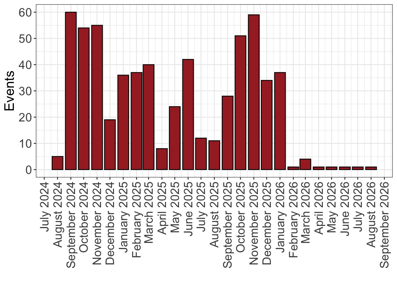
As of 21 January 2026, there were 645 events listed on the Rooted Calendar. Figure 1 shows that the catalogue covers events over the preceding 18 months as well as a handful upcoming events.
Click to expand/collapse the code
library(ggplot2)
library(lubridate)

events_bars <- ER %>%
  mutate(month_period = floor_date(event_date, unit = "1 months")) %>%
  count(month_period) %>%
  ggplot(aes(x = month_period, y = n)) +
  geom_col(colour="black", fill="brown") +
  scale_x_date("", date_labels = "%B %Y", date_breaks = "1 month") +
  scale_y_continuous("Events",
    breaks = seq(0, 70, by = 10),
    minor_breaks = seq(0, 70, by = 5)
  ) +
  theme_bw() +
  theme(
    axis.text.x = element_text(angle = 90, hjust = 1, vjust = 0.5, size = 15),
    axis.text.y = element_text(size = 15),
    axis.title.y = element_text(size = 17)
  )
The operators of the Rooted Calendar seem to have covered quite a few organisations. 83 are represented in the data, though not all of these have organised an event (yet): 60 have organised at least one event. Figure 2 depicts this diffuse spread of organisers.
Click to expand/collapse the code
library(forcats)
library(ggiraph)

piechartER <- ER %>%
  mutate(group = fct_lump_n(group, n = 10, other_level = "Other")) %>%
  count(group) %>%
  mutate(
    group = fct_reorder(group, n, .desc = TRUE),
    group = fct_relevel(group, "Other", after = Inf)
  ) %>%
  ggplot(aes(x = "", y = n, fill = group, tooltip = paste(group, ": ", n))) +
  geom_bar_interactive(stat = "identity", width = 1, color = "white") +
  coord_polar(theta = "y") +
  scale_fill_manual(values = c(
    "#1b9e77",
    "#d95f02",
    "#7570b3",
    "#e7298a",
    "#66a61e",
    "#e6ab02",
    "#a6761d",
    "#1f78b4",
    "#b2df8a",
    "#fb9a99",
    "grey70"
  )) +
  labs(
    title = "Top 10 Event Organisers",
    x = NULL,
    y = NULL
  ) +
  theme_void() +
  theme(
    legend.title = element_blank(),
    legend.text = element_text(size = 12)
  )

piechartERinteractive <- girafe(ggobj = piechartER,
       options = list(
    opts_hover(
      css = girafe_css(
        css = '',
        area = 'stroke: black; fill: black;'
      )
    )
))The majority of these events were the initiative of one organisation. However, there is also extensive collaboration between the organisations listed on the Rooted Calendar. 158 events were the product of collaboration between two or more organisations. In this way the Rooted Calendar provides some insight into the networks of interaction between French far-right organisations.
Events and their organisers
The Rooted Calendar data allows for the construction of a classic ‘affiliation network’ (or two-mode network) with nodes for the events organised and the actors organising them. Figure 3 shows a projection of this network, with circular blue nodes representing events and square red nodes representing the organisations connected to those events (and through them to other organisations).
Click to expand/collapse the code
library(stringr)

## split the column of named organisers

ER_clean <- ER %>%
  mutate(
    event_id = row_number(),
    organisateurs = str_remove_all(organisateurs, "\\s*;\\s*$") # remove trailing ;
  ) %>%
  separate_rows(organisateurs, sep = ";") %>%
  mutate(
    organisateurs = str_trim(organisateurs)
  )

library(igraph)

ER_edges_2mode <- ER_clean %>% select(event_id, organisateurs)

ER_graph_2mode <- graph_from_data_frame(ER_edges_2mode, directed = FALSE)

## distinguish node types (for two-mode plotting)
V(ER_graph_2mode)$type <- V(ER_graph_2mode)$name %in% ER_clean$organisateurs

V(ER_graph_2mode)$shape <- ifelse(V(ER_graph_2mode)$type, "square", "circle")
V(ER_graph_2mode)$size <- ifelse(V(ER_graph_2mode)$type, 6, 3)

## labels for only the organisations
vertex_labels <- ifelse(V(ER_graph_2mode)$type == TRUE, V(ER_graph_2mode)$name, NA)

par(mar = c(0, 0, 0, 0))

# plot(
#   ER_graph_2mode,
#   vertex.color = ifelse(V(ER_graph_2mode)$type, "tomato", "skyblue"),
#   vertex.label.cex = 0.6,
#   # vertex.size = 6,
#   layout = layout_as_bipartite(ER_graph_2mode)
# )

# plotER_graph_2mode <- plot(
#   ER_graph_2mode,
#   vertex.color = ifelse(V(ER_graph_2mode)$type, "tomato", "skyblue"), ## organisations, events
#   edge.color = "red",
#   vertex.label = vertex_labels,
#   vertex.label.family="Helvetica",
#   vertex.label.color=c("blue"),
#   vertex.label.font=2, # Font: 1plain, 2bold, 3italic, 4bold italic, 5symbol
#   vertex.label.cex=0.8,
#   # vertex.size = 6,
#   layout = layout_with_fr(ER_graph_2mode)
# )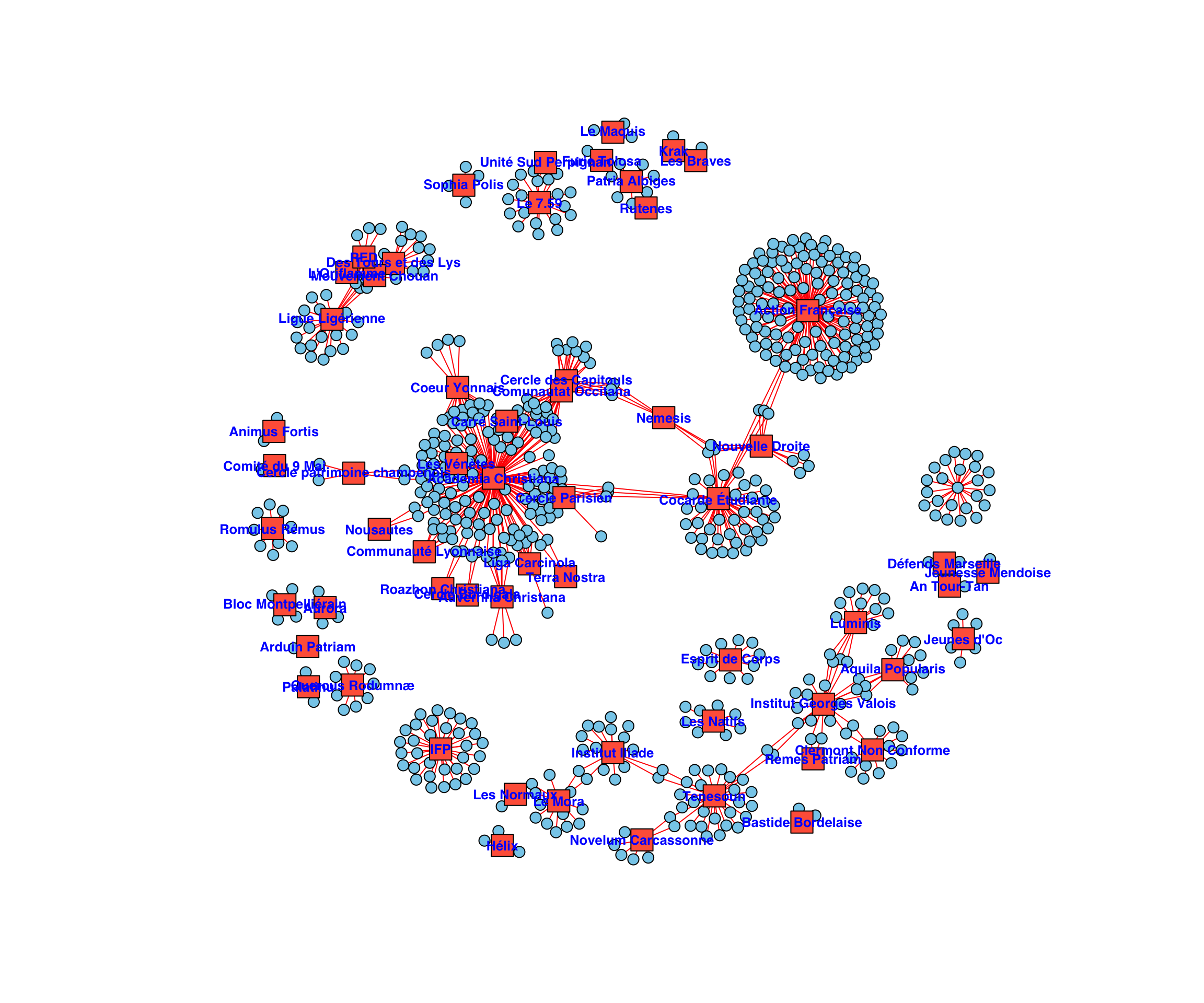
Some organisations seem to keep to themselves. For example, none of the events organised by the IFP (l’Institut de Formation Politique), run by Alexandre Pesey, were co-organised with another organisation listed by the Rooted Calendar. Others seldom collaborate: Action Française, one of the oldest and largest French far-right organisations, is a highly active event organiser—the most prolific in the Rooted Calendar (Figure 2)—but only rarely co-organises events. Still others are veritable hubs of interactivity. At the centre of the biggest cluster in Figure 3 is Academia Christiana, a radical right organisation that was at one point (in late 2023) faced the possibility of organisational proscription by the French state.
Inter-organisation collaboration
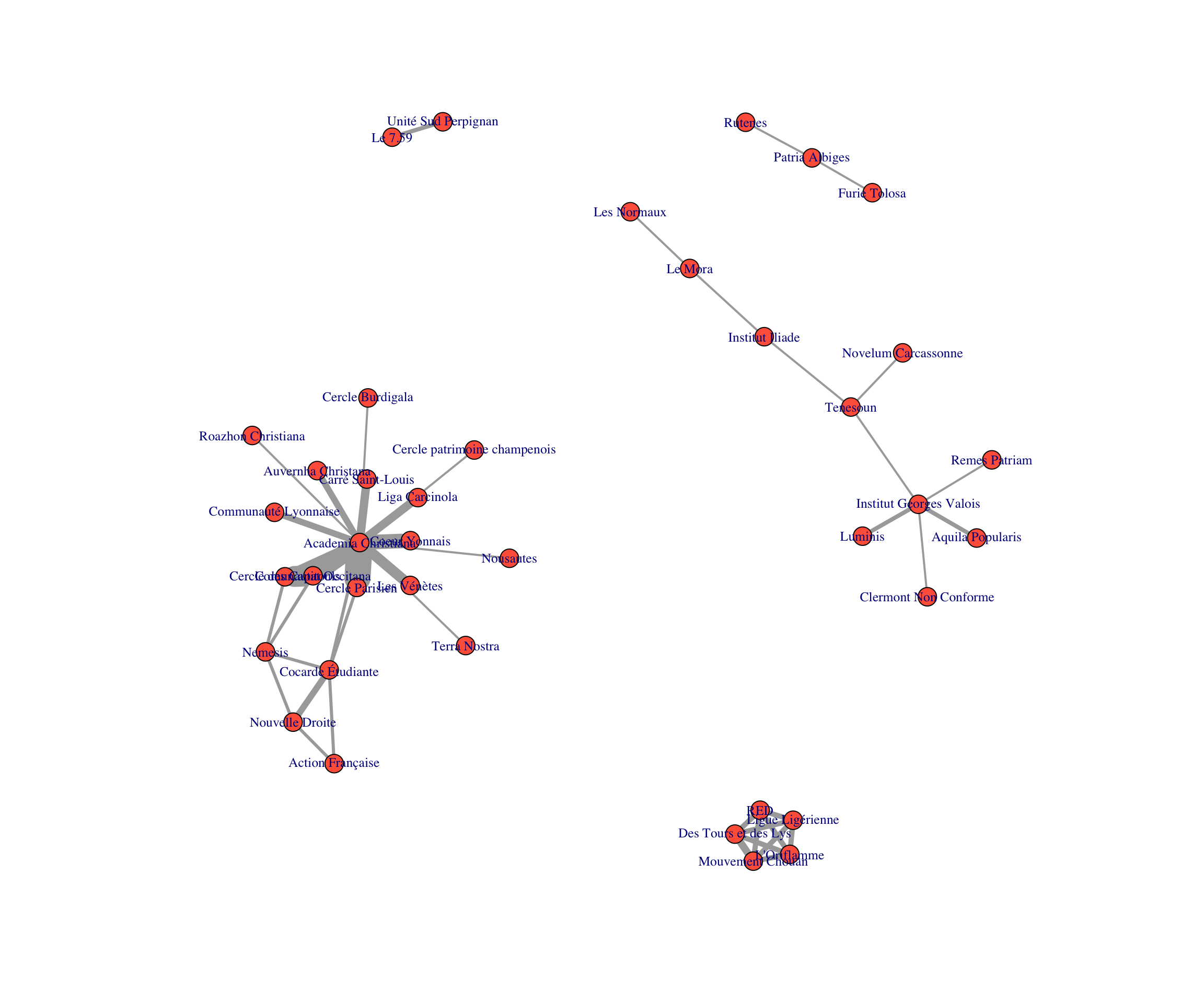
We can simplify the network graphic by focusing on the links between organisations, created by their collaboration on events. (This is the common procedure of projecting a two-mode network as a one-mode network.) Figure 4 shows a network composed just of organisations, with the edges (links between nodes) weighted according to the number of times the organisations co-organised events. Here, the different clusters of organisations that work together is clearer.
Click to expand/collapse the code
multi_events <- ER_clean %>%
  group_by(event_id) %>%
  filter(n() > 1) %>%
  ungroup()

edges_multi <- multi_events %>%
  select(event_id, organisateurs)

g_multi <- graph_from_data_frame(edges_multi, directed = FALSE)

V(g_multi)$type <- V(g_multi)$name %in% multi_events$organisateurs

proj <- bipartite_projection(g_multi)

g_org <- proj$proj2   # organisation projection

# plot(
#   g_org,
#   vertex.color = "tomato",
#   vertex.size = 5, # igraph::degree(g_org) * 2,
#   vertex.label.cex = 0.8,
#   edge.width = E(g_org)$weight
# )
The ggraph package makes it a bit easier to add in some extra elements to the plot. Figure 5 shows those weights of connection as well as sizing nodes by their centrality.
Click to expand/collapse the code
library(dplyr)
library(tidyr)
library(stringr)
library(tidygraph)
library(ggraph)
library(igraph)

ER_clean <- ER %>%
  mutate(
    event_id = row_number(),
    organisateurs = str_remove_all(organisateurs, "\\s*;\\s*$")
  ) %>%
  separate_rows(organisateurs, sep = ";") %>%
  mutate(organisateurs = str_trim(organisateurs))

multi_events <- ER_clean %>%
  group_by(event_id) %>%
  filter(n() > 1) %>%
  ungroup()

edges <- multi_events %>%
  select(event_id, organisateurs)

g_bip <- graph_from_data_frame(edges, directed = FALSE)

# Mark node types (TRUE = organisation)
V(g_bip)$type <- V(g_bip)$name %in% multi_events$organisateurs

proj <- bipartite_projection(g_bip)

g_org_igraph <- proj$proj2

g_org <- tidygraph::as_tbl_graph(g_org_igraph)

# Edge width = number of shared events
# Node size = number of collaborators
# Labels repel automatically
ggplot_g_org <- ggraph(g_org, layout = "fr") + # Fruchterman-Reingold layout OR 'stress'
  geom_edge_link(aes(width = weight), alpha = 0.4) +
  geom_node_point(aes(size = centrality_degree()), color = "tomato") +
  geom_node_text(aes(label = name), repel = TRUE, size = 3) +
  scale_edge_width(range = c(0.2, 2)) +
  theme_graph()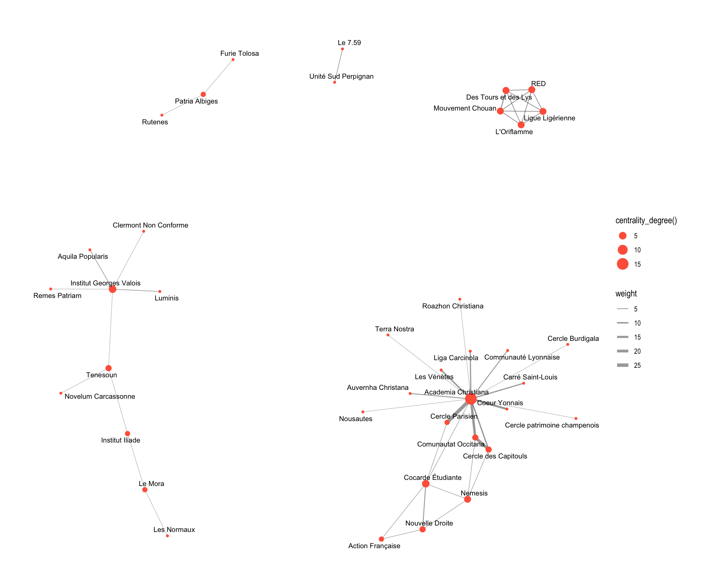
Figure 6 merely provides an interactive version of this organisation-to-organisation network, adding the classification (‘type’) listed on the Rooted Calendar.
Click to expand/collapse the code
## full set of options: https://datastorm-open.github.io/visNetwork/igraph.html
library(visNetwork)
## Basic vis
# visNetwork::visIgraph(g_org, physics = FALSE, smooth = TRUE, idToLabel = TRUE)

g_org_VN <- toVisNetworkData(g_org)

g_org_VN$edges$value <- g_org_VN$edges$weight # to automatically weight the edges

### adding shape -- if not using visGroups
# g_org_VN$nodes$shape <- "diamond"

# to auto-size the nodes
g_org_VN$nodes <- g_org_VN$nodes %>%
  left_join(
    g_org_VN$edges %>%
      count(from, name = "value"),
    by = c("id" = "from")
  ) %>%
  mutate(value = ifelse(is.na(value), 0, value))

## add in the 'type' of organisation
ER_unique <- ER %>%
  group_by(group) %>%
  summarise(type = first(type), .groups = "drop")

g_org_VN$nodes <- g_org_VN$nodes %>%
  left_join(ER_unique, by = c("id" = "group"))

g_org_VN$nodes <- g_org_VN$nodes %>% dplyr::rename(group = type)


### adding colour therefrom -- if not using visGroups
# g_org_VN$nodes <- g_org_VN$nodes %>%
#   mutate(
#     color=case_when(
#       type=="Formation" ~ "darkred",
#       type=="Activisme" ~ "forestgreen",
#       type=="Communauté"~ "goldenrod",
#       TRUE ~ "lightblue"
#     )
#   )

plot_g_org_VN <- visNetwork(nodes=g_org_VN$nodes, edges=g_org_VN$edges,
           physics = TRUE, smooth = TRUE, idToLabel = TRUE) %>% # , height = "500px"
  visIgraphLayout() %>% # layout = "layout_in_circle"
  visNodes(scaling = list(min = 15, max = 50)) %>%
  visGroups(groupname = "Activisme", color = "forestgreen", shape = "triangle") %>%
  visGroups(groupname = "Communauté", color = "goldenrod", shape = "diamond") %>%
  visGroups(groupname = "Formation", color = "darkred", shape = "square") %>%
  visEdges(scaling = list(min = 5, max = 30),
           color = list(color = "navy", highlight = "red")) %>%
  visOptions(selectedBy = "group",
             highlightNearest = list(enabled = T, hover = T),
             nodesIdSelection = T) %>%
  visPhysics(stabilization = FALSE) %>%
  visLegend(width = 0.2, position = "right", main = "Group type") %>%

  # visConfigure(enabled = TRUE) %>%
  visLayout(randomSeed = 12) # to have always the same network


g_org_VN$nodes$idx <- gsub(" ", "", g_org_VN$nodes$id)
g_org_VN$nodes$idx <- gsub("é", "e", g_org_VN$nodes$idx)
g_org_VN$nodes$idx <- gsub("è", "e", g_org_VN$nodes$idx)
g_org_VN$nodes$idx <- gsub("É", "E", g_org_VN$nodes$idx)
g_org_VN$nodes$idx <- gsub("ç", "c", g_org_VN$nodes$idx)

g_org_VN$nodes <- g_org_VN$nodes %>%
  mutate(shape = c("circularImage"), # "image", "circularImage"
         )

# g_org_VN$nodes <- g_org_VN$nodes %>%
#   mutate(image = paste0("FRA_fr_logos_nospace/", idx, ".png"))
path_to_images <- "https://raw.githubusercontent.com/michaelczeller/data-open/refs/heads/main/FRA_fr_logos_nospace/"

g_org_VN$nodes <- g_org_VN$nodes %>%
    mutate(image = paste0(path_to_images, idx, ".png"))


# g_org_VN$nodes <- g_org_VN$nodes %>%
#   dplyr::select(id, shape, image, label)


plot_g_org_VN_img <- visNetwork(nodes=g_org_VN$nodes, edges=g_org_VN$edges,
           physics=TRUE, smooth=TRUE, idToLabel=TRUE, width="100%") %>%
  visIgraphLayout() %>%
  visNodes(shapeProperties = list(useBorderWithImage = TRUE),
           scaling = list(min = 30, max = 70)) %>%
  visGroups(groupname="Activisme", color="forestgreen") %>% #, shape="triangle"
  visGroups(groupname="Communauté", color="goldenrod") %>% # , shape="diamond"
  visGroups(groupname="Formation", color="darkred") %>% # , shape="square"
  visLayout(randomSeed = 2) %>%
  visEdges(scaling = list(min = 5, max = 30),
           color = list(color = "navy", highlight = "red")) %>%
  visOptions(selectedBy = "group",
             highlightNearest = list(enabled = T, hover = T),
             nodesIdSelection = T) %>%
  visPhysics(stabilization = FALSE) %>%
  visLegend(width = 0.2, position = "right", main = "Group type") %>%
visLayout(randomSeed = 12) # to have always the same network network measures
With such a limited, curated set of events and collaborations, it does not make much sense to provide network-wide metrics. For those a fuller dataset is needed. But we can meaninfully quantify some node metrics:
- degree centrality: number of direct connections a node has. High degree means the node is directly connected to many others.
- strength: sum of the weights of a node’s connections. High strength means the node has strong or high-volume connections.
- betweenness centrality: how often a node lies on the shortest paths between other nodes. High betweenness means the node acts as a bridge or broker between different parts of the network.
- closeness centrality: how close a node is to all other nodes in the network (by shortest paths). High closeness means the node can connect to others quickly (i.e., few steps away).
- Eigenvector centrality: a node’s importance based on both (i) how many connections it has and (ii) how important its neighbours are. High eigenvector centrality means the node is connected to other well-connected nodes.
- pagerank: the probability that a random walker moving through the network would land on a given node. High PageRank means the node is frequently reached via incoming links from important nodes.
Click to expand/collapse the code
library(DT)

g_org <- g_org %>%
  activate(nodes) %>%
  mutate(
    degree = centrality_degree(),
    strength = centrality_degree(weights = weight),
    betweenness = centrality_betweenness(weights = weight, normalized = TRUE),
    closeness = centrality_closeness(),
    eigenvector = centrality_eigen(weights = weight),
    pagerank = centrality_pagerank(weights = weight)
  )

centrality_df <- g_org %>%
  activate(nodes) %>%
  as_tibble() %>%
  select(name, degree, strength, betweenness,
         closeness, eigenvector, pagerank)

centrality_df_tab <- centrality_df %>%
  mutate_at(vars(betweenness, closeness, eigenvector, pagerank),
            funs(round(., 3)))

dt_node_measures <- datatable(centrality_df_tab, rownames = FALSE,
          caption = 'Node metrics.',
          filter = 'top', options = list(pageLength = 10, autoWidth = TRUE)) %>%
  formatStyle(columns = c(1:ncol(centrality_df_tab)), fontSize = '70%')
Network evolution
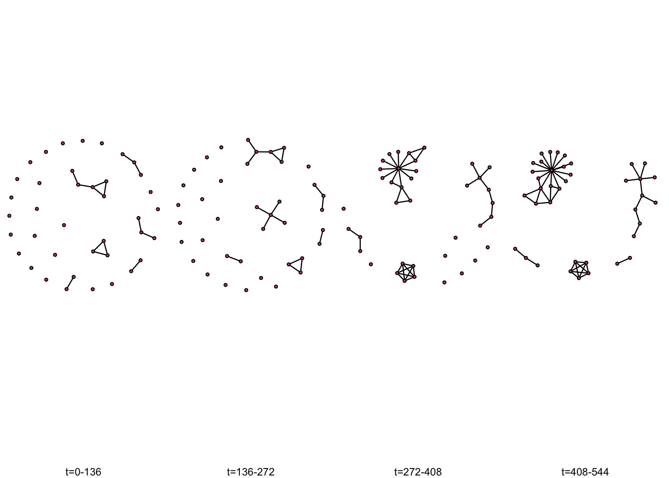
Crucial for assessing how organisations interact, pool resources, and collaborate is the ability to track the evolution of this network. There are several visual ways to do this. For example, one can take snapshots of the network in different periods (again assuming that an enduring link is created between organisations when they co-participate in an event).
Click to expand/collapse the code
## ~~~~~~~~~~~~~~~~~~~~~~~~~~~~~~~~~~~~~~~~~~~~~~~~~~~
## CUMULATIVE (MONOTONIC) EDGE PROCESS (once a tie appears it never disappears)
library(ndtv)
library(networkDynamic)
library(dplyr)
library(tidyr)
library(purrr)
library(stringr)

df <- ER %>%
  select(group, type, event_date, loc, organisateurs) %>%
  mutate(
    organisateurs = str_split(organisateurs, ";"),
    organisateurs = map(organisateurs, ~ str_trim(.x)),
    organisateurs = map(organisateurs, ~ .x[.x != ""]) # remove empty
  ) %>%
  filter(lengths(organisateurs) > 1) %>%   # keep only multi आयोज
  mutate(event_id = row_number())

## create nodes dataframe
nodes_df <- df %>%
  select(group, type, organisateurs) %>%
  unnest(organisateurs) %>%
  distinct(organisateurs, .keep_all = TRUE) %>%
  mutate(
    id = row_number(),
    type.label = type
  ) %>%
  ##create a numeric encoding for each unique type.label
  mutate(type = as.integer(factor(type.label))) %>%
  rename(organisation = organisateurs) %>%
  select(id, organisation, type, type.label) %>%
  as.data.frame()

nodes_df <- nodes_df %>%
  mutate(
    org.label=case_when(
      organisation=="Academia Christiana" ~ "AC",
      organisation=="Les Vénètes" ~ "Vénètes",
      organisation=="Coeur Yonnais" ~ "CY",
      organisation=="Cercle Parisien" ~ "CP",
      organisation=="Cercle Burdigala" ~ "CB",
      organisation=="Carré Saint-Louis" ~ "CSL",
      organisation=="Cercle des Capitouls" ~ "CdC",
      organisation=="Comunautat Occitana" ~ "CO",
      organisation=="Liga Carcinola" ~ "LC",
      organisation=="Auvernha Christana" ~ "AuvC",
      organisation=="Communauté Lyonnaise" ~ "CL",
      organisation=="Terra Nostra" ~ "TN",
      organisation=="Roazhon Christiana" ~ "RC",
      organisation=="Cocarde Étudiante" ~ "CE",
      organisation=="Cercle patrimoine champenois" ~ "CPC",
      organisation=="Action Française" ~ "AF",
      organisation=="Nouvelle Droite" ~ "ND",
      organisation=="Aquila Popularis" ~ "AP",
      organisation=="Institut Georges Valois" ~ "IGV",
      organisation=="Clermont Non Conforme" ~ "CNC",
      organisation=="Des Tours et des Lys" ~ "DTDL",
      organisation=="Ligue Ligérienne" ~ "LL",
      organisation=="L'Oriflamme" ~ "Oriflamme",
      organisation=="Mouvement Chouan" ~ "Chouan",
      organisation=="Furie Tolosa" ~ "FT",
      organisation=="Patria Albiges" ~ "PA",
      organisation=="Remes Patriam" ~ "RP",
      organisation=="Institut Iliade" ~ "II",
      organisation=="Unité Sud Perpignan" ~ "USP",
      organisation=="Les Normaux" ~ "Normaux",
      organisation=="Novelum Carcassonne" ~ "NC",
      TRUE ~ organisation
    )
  )

## split the column of named organisers
ER_clean <- ER %>%
  mutate(
    event_id = row_number(),
    organisateurs = str_remove_all(organisateurs, "\\s*;\\s*$") # remove trailing ;
  ) %>%
  separate_rows(organisateurs, sep = ";") %>%
  mutate(
    organisateurs = str_trim(organisateurs)
  )

# split organisers into list
ER_pairs <- ER_clean %>%
  mutate(group_list = strsplit(organisateurs, ",\\s*")) %>%
  select(event_id, event_date, group_list) %>%
  unnest(group_list)

## create all pairwise combinations per event, keeping only events with more than 2 organisers and making edges undirected and consistent
ER_edges <- ER_pairs %>%
  group_by(event_id, event_date) %>%
  summarise(
    group_list = list(unique(group_list)),  # remove duplicates within event
    n_groups = length(group_list[[1]]),
    .groups = "drop"
  ) %>%
  filter(n_groups >= 2) %>%
  rowwise() %>%
  mutate(
    pairs = list(t(combn(group_list, 2)))
  ) %>%
  unnest(pairs) %>%
  mutate(
    head = pmin(pairs[,1], pairs[,2]),
    tail = pmax(pairs[,1], pairs[,2])
  ) %>%
  select(head, tail, event_date) %>%
  ## get rid of duplicated rows
  distinct(.keep_all = TRUE)

### compute weights
## final weight (total collaborations)
ER_edges <- ER_edges %>%
  group_by(head, tail) %>%
  mutate(weight_fin = n()) %>%
  ungroup()
## Accumulated weight over time
ER_edges <- ER_edges %>%
  arrange(head, tail, event_date) %>%
  group_by(head, tail) %>%
  mutate(weight_acc = row_number()) %>%
  ungroup()

library(network)

netER <- network(ER_edges,  vertex.attr=nodes_df, matrix.type="edgelist",
                loops=T, multiple=T, ignore.eval = F)

netER %n% "net.name" <- "French radical right network" #  network attribute
# netER %v% "type" # Node attribute
# netER %v% "type.label" # Node attribute
# netER %v% "org.label" # Node attribute
# netER %e% "event_date"  # Edge attribute
# netER %e% "weight_fin"  # Edge attribute
# netER %e% "weight_acc"  # Edge attribute

netER %v% "col" <- c("darkred", "goldenrod", "forestgreen")[netER %v% "type"]
# plot(netER, vertex.cex=3, vertex.col="col")

# ## PLOT OPTIONS: https://cran.r-project.org/web/packages/network/network.pdf
# plot(netER, usearrows = F,
#      vertex.cex=2, vertex.col="col", vertex.lwd=0.2,
#      displaylabels = T, boxed.labels=F, label.cex=0.5, label.col="darkred",
#      edge.lwd = (netER %e% "weight_fin")*2, edge.col="blue")

# ## Note that - as in igraph - the plot returns the node position coordinates. You can use them in other plots using the coord parameter.
# l <- plot(netER, usearrows = F,
#      vertex.cex=2, vertex.col="col", vertex.lwd=0.2,
#      displaylabels = T, boxed.labels=F, label.cex=0.5, label.col="darkred",
#      edge.lwd = (netER %e% "weight_fin")*2, edge.col="blue")
# plot(netER, usearrows = F,
#      vertex.cex=2, vertex.col="col", vertex.lwd=0.2,
#      displaylabels = T, boxed.labels=F, label.cex=0.5, label.col="darkred",
#      edge.lwd = (netER %e% "weight_fin")*2, edge.col="blue",
#      coord=l)

## The network package also offers the option to edit a plot interactively, by setting the parameter interactive=T:
# plot(netER, usearrows = F,
#      vertex.cex=3, vertex.col="col", vertex.lwd=0.2,
#      displaylabels = T, boxed.labels=F, label.cex=0.5, label.col="darkred",
#      edge.lwd = (netER %e% "weight_fin"), edge.col="blue",
#      interactive=T)

edge_spells <- ER_edges %>%
  rename(onset_date=event_date) %>% dplyr::select(head, tail, onset_date, weight_acc, weight_fin) # , weight_acc, weight_fin

### set end at latest date in dataset (there may be NAs in dataset)
end_time <- max(ER_edges$event_date, na.rm = TRUE)

ER_edges <- ER_edges %>%
  rename(from = head,
         to = tail,
         weight=weight_fin) %>%
  mutate(type="cooperation") %>%
  dplyr::select(from, to, type, weight, weight_acc) %>% # , weight_acc
  as.data.frame()

edge_spells <- edge_spells %>% mutate(terminus_date = end_time)

## convert dates to numeric time
origin <- min(edge_spells$onset_date)

edge_spells <- edge_spells %>%
  mutate(
    onset = as.numeric(onset_date - origin),
    terminus = as.numeric(terminus_date - origin)
  ) %>%
  dplyr::select(onset, terminus, head, tail, weight_acc, weight_fin) # , onset_date, terminus_date, weight_acc, weight_fin

# ## map groups to numeric IDs
nodes <- sort(unique(c(edge_spells$tail, edge_spells$head)))

node_ids <- data.frame(
  name = nodes,
  id = seq_along(nodes)
)

edge_spells_clean <- edge_spells %>%
  left_join(node_ids, by = c("tail" = "name")) %>%
  rename(tail_id = id) %>%
  left_join(node_ids, by = c("head" = "name")) %>%
  rename(head_id = id) %>%
  rename(tail_name = tail,
         head_name = head)

edge_spells_clean <- edge_spells_clean %>%
  select(onset, terminus, head_id, tail_id, head_name, tail_name, weight_acc, weight_fin) %>% #
  mutate(
    onset = as.numeric(onset),
    terminus = as.numeric(terminus),
    head = as.integer(head_id),
    tail = as.integer(tail_id)
  ) %>%
  select(onset, terminus, head, tail, weight_acc, weight_fin) %>% # , head_name, tail_name, weight_acc, weight_fin
  as.data.frame()

## recast termini for dynamic edge attribute of accumulating weight
edge_spells_fixed <- edge_spells_clean %>%
  arrange(head, tail, onset) %>%
  group_by(head, tail) %>%
  mutate(
    terminus = lead(onset, default = first(terminus))
  ) %>%
  ungroup() %>%
  as.data.frame()

col_fun <- colorRampPalette(c("#53adcb", "red"))
colors_12 <- col_fun(12)
edge_spells_fixed$cols <- colors_12[edge_spells_fixed$weight_acc]

## thicker edges
edge_spells_fixed$weight_acc2 <- (1.5*edge_spells_fixed$weight_acc)

# str(edge_spells_fixed)
# summary(edge_spells_fixed)

node_ids <- node_ids %>%
  mutate(
    onset = min(edge_spells_fixed$onset),
    terminus = max(edge_spells_fixed$terminus)
  ) %>%
  rename(vertex.id = id) %>%
  dplyr::select(onset, terminus, vertex.id) # , name

## create networkDynamic
CumulativeERnet <- networkDynamic(vertex.spells = node_ids,
                                  edge.spells = edge_spells_fixed, #[, c(1:8)]
                                  create.TEAs=T,
                                  edge.TEA.names=c('weight_acc',
                                                   'weight_fin',
                                                   'cols',
                                                   'weight_acc2'),
                                  verbose = F
                                  )

# activate.edge.attribute(CumulativeERnet,'width',1,onset=0,terminus=200)
# activate.edge.attribute(CumulativeERnet,'width',5,onset=200,terminus=400)
# activate.edge.attribute(CumulativeERnet,'width',10,onset=400,terminus=Inf)

par(mar = c(1, 0.2, 0.2, 0.2))

# filmstrip(CumulativeERnet, displaylabels=F, mfrow=c(1, 4),
#           slice.par=list(start=0, end=540, interval=136,
#                          aggregate.dur=136, rule='any'))

compute.animation(CumulativeERnet,
                  animation.mode = "kamadakawai",
                  # weight.attr = "weight_acc", ## adding this messes with layout
                  slice.par=list(start=0, end=539, interval=1,
                         aggregate.dur=1, rule='all'), verbose = F)

# ## render.d3movie(CumulativeERnet,displaylabels=TRUE)
# timePrism(CumulativeERnet, at = c(200,280,400, 530))
#
# proximity.timeline(CumulativeERnet, mode='sammon',
#                    default.dist=10,
#                    # labels.at=c(1,16,25),
#                    onsets = 300,
#                    label.cex=0.7,
#                    vertex.col=c(rep('gray',14),'green','blue'),
#                    labels.at=540
#                    )

library(scales)

# render.d3movie(CumulativeERnet, usearrows = F,
#        displaylabels = T, label=netER %v% "org.label",
#        bg="#F0EAD6", vertex.border="#333333",
#        vertex.cex = function(slice){ rescale(degree(slice), to = c(1, 3)) },
#        # vertex.cex = rescale(degree(netER), to = c(2, 5)),
#        vertex.col = netER %v% "col",
#        edge.lwd = 'weight_acc2',
#        # edge.lwd = (rescale(netER %e% "weight_fin", to = c(1, 10))),
#        edge.col = 'cols',
#        # edge.col = '#53adcb', # 'lightblue',
#        # edge.col=function(slice){rgb(slice%e%'width_acc'/10,0,0)},
#        vertex.tooltip=paste("<b>Name:</b>", (netER %v% "organisation") , "<br>",
#                               "<b>Type:</b>", (netER %v% "type.label")),
#        edge.tooltip = function(slice) {
#          w_acc <- slice %e% "weight_acc"
#          w_fin <- slice %e% "weight_fin"
#          paste0("<b>No. of collaborations at time:</b> ", w_acc,
#                 "<br><b>Final No. of collaborations:</b> ", w_fin)
#          },
#        launchBrowser=F, filename="French-RR-Network-Dynamic.html",
#        render.par=list(tween.frames = 10, show.time = T),
#        plot.par=list(mar=c(0,0,0,0)) ) # , output.mode='inline')

## output.mode='inline' to embed the plot in a markdown document
Figure 7 shows the network at four different stages.
Similarly, Figure 8 shows the development of the network.
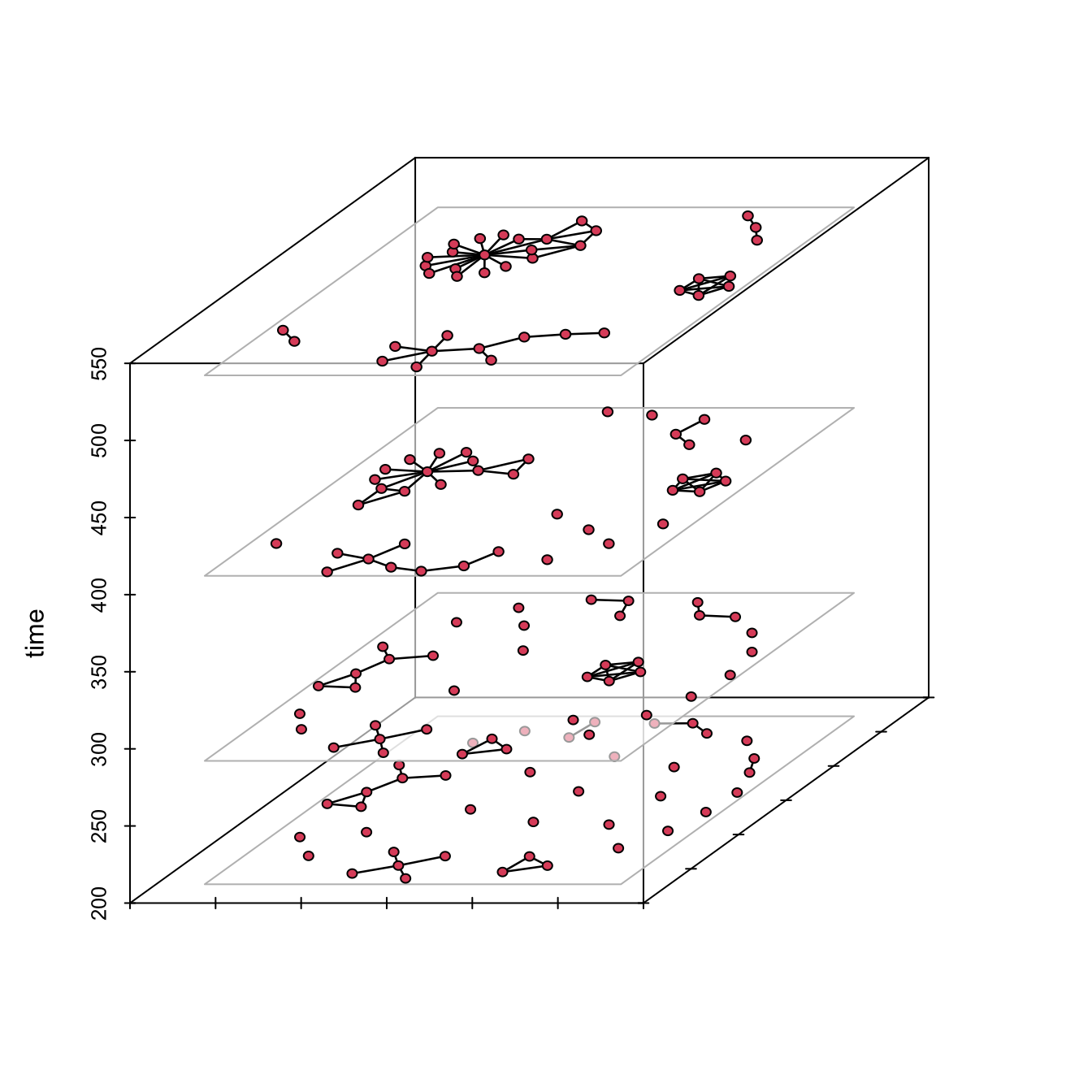
But probably the most effective way of showing this evolution (certainly the most granular) is to animate the day-by-day accumulation of links between organisations based on co-participation in events, as below.
Data
Raw data scraped from https://en-racine.org/
scraping code
Click to expand/collapse the code
library(tibble)
library(rvest)
library(purrr)
library(dplyr)
library(tidyr)
library(stringr)

## a bit hacky, but since the website is in JS, one can look at the
## developer side of the site and manually pull out the list of
## organisations and their 'type'

text_data <- "Academia Christiana
Formation
Action Française
Activisme
Alamans Strasbourg
Activisme
Allobroges
Activisme
Animus Fortis
Activisme
An Tour-Tan
Activisme
Aquila Popularis
Activisme
Arduin Patriam
Activisme
Arlé
Activisme
Auctorum
Activisme
Audace
Activisme
Aurelianorum Corda
Activisme
Aurora
Activisme
Auvernha Christana
Communauté
Bastide Bordelaise
Activisme
Bloc Montpelliérain
Activisme
Carré Saint-Louis
Communauté
Cénomans
Activisme
Cercle Burdigala
Communauté
Cercle des Capitouls
Formation
Cercle Parisien
Communauté
Cercle patrimoine champenois
Communauté
Cervus Picardae
Activisme
Clermont Non Conforme
Activisme
Cocarde Étudiante
Activisme
Coeur Yonnais
Communauté
Columna
Activisme
Comité du 9 Mai
Activisme
Communauté Lyonnaise
Communauté
Comunautat Occitana
Communauté
Défends Marseille
Activisme
Des Tours et des Lys
Activisme
Esprit de Corps
Communauté
Forez Front
Activisme
Fraternité Comtoise
Activisme
Furie Tolosa
Activisme
Hélix
Activisme
Heritage Lyon
Activisme
Heritage Savoie
Activisme
IFP
Formation
Institut Georges Valois
Formation
Institut Iliade
Formation
Jeunes d'Oc
Activisme
Jeunesse Mendoise
Activisme
Krak
Activisme
L'Alérion
Activisme
Le 7.59
Communauté
Le Maquis
Activisme
Le Mora
Communauté
Les Bayards
Activisme
Les Braves
Communauté
Les Hesperianoí
Communauté
Les Natifs
Activisme
Les Normaux
Activisme
Les Téméraires
Communauté
Les Vénètes
Communauté
Liga Carcinola
Communauté
Ligue Ligérienne
Activisme
L'Oriflamme
Activisme
Luminis
Activisme
Meduana Noctua
Activisme
Mouvement Chouan
Activisme
Nemesis
Activisme
Neuer Wanderbund
Activisme
Nousautes
Communauté
Nouvelle Droite
Activisme
Novelum Carcassonne
Activisme
Opus
Communauté
Palatinu
Activisme
Patria Albiges
Activisme
Quercus Rodumnæ
Communauté
RED
Activisme
Remes Patriam
Activisme
Roazhon Christiana
Communauté
Romulus Rémus
Formation
Rutenes
Activisme
Sophia Polis
Formation
Souvenir Normand
Communauté
Tenesoun
Activisme
Terra Nostra
Communauté
Unité Sud Perpignan
Activisme
Valyor
Activisme
Vosegus Epinal
Activisme
"

lines <- unlist(strsplit(text_data, "\n"))

## remove leading or trailing whitespace from each line
lines <- trimws(lines)

# create tibble by alternating odd (group) and even (type) lines
df <- tibble(
  group = lines[seq(1, length(lines), by = 2)],
  type = lines[seq(2, length(lines), by = 2)]
)

## similarly hacky, one can pull out the organisation pages from the
## developer side of the website

Pages <- c("https://en-racine.org/association/1-academia-christiana",
          "https://en-racine.org/association/5-action-francaise",
          "https://en-racine.org/association/101-alamans-strasbourg",
          "https://en-racine.org/association/71-allobroges",
          "https://en-racine.org/association/4-animus-fortis",
          "https://en-racine.org/association/2-an-tour-tan",
          "https://en-racine.org/association/6-aquila-popularis",
          "https://en-racine.org/association/91-arduin-patriam",
          "https://en-racine.org/association/8-arle",
          "https://en-racine.org/association/9-auctorum",
          "https://en-racine.org/association/83-audace",
          "https://en-racine.org/association/66-aurelianorum-corda",
          "https://en-racine.org/association/10-aurora",
          "https://en-racine.org/association/73-auvernha-christana",
          "https://en-racine.org/association/30-bastide-bordelaise",
          "https://en-racine.org/association/11-bloc-montpellierain",
          "https://en-racine.org/association/96-carre-saint-louis",
          "https://en-racine.org/association/99-cenomans",
          "https://en-racine.org/association/98-cercle-burdigala",
          "https://en-racine.org/association/67-cercle-des-capitouls",
          "https://en-racine.org/association/70-cercle-parisien",
          "https://en-racine.org/association/77-cercle-patrimoine-champenois",
          "https://en-racine.org/association/82-cervus-picardae",
          "https://en-racine.org/association/63-clermont-non-conforme",
          "https://en-racine.org/association/14-cocarde-etudiante",
          "https://en-racine.org/association/65-coeur-yonnais",
          "https://en-racine.org/association/86-columna",
          "https://en-racine.org/association/69-comite-du-9-mai",
          "https://en-racine.org/association/87-communaute-lyonnaise",
          "https://en-racine.org/association/16-comunautat-occitana",
          "https://en-racine.org/association/18-defends-marseille",
          "https://en-racine.org/association/17-des-tours-et-des-lys",
          "https://en-racine.org/association/20-esprit-de-corps",
          "https://en-racine.org/association/79-forez-front",
          "https://en-racine.org/association/21-fraternite-comtoise",
          "https://en-racine.org/association/22-furie-tolosa",
          "https://en-racine.org/association/24-helix",
          "https://en-racine.org/association/94-heritage-lyon",
          "https://en-racine.org/association/95-heritage-savoie",
          "https://en-racine.org/association/68-ifp",
          "https://en-racine.org/association/25-institut-georges-valois",
          "https://en-racine.org/association/26-institut-iliade",
          "https://en-racine.org/association/27-jeunes-doc",
          "https://en-racine.org/association/90-jeunesse-mendoise",
          "https://en-racine.org/association/92-krak",
          "https://en-racine.org/association/28-lalerion",
          "https://en-racine.org/association/46-le-759",
          "https://en-racine.org/association/32-le-maquis",
          "https://en-racine.org/association/33-le-mora",
          "https://en-racine.org/association/80-les-bayards",
          "https://en-racine.org/association/34-les-braves",
          "https://en-racine.org/association/35-les-hesperianoi",
          "https://en-racine.org/association/36-les-natifs",
          "https://en-racine.org/association/37-les-normaux",
          "https://en-racine.org/association/38-les-temeraires",
          "https://en-racine.org/association/85-les-venetes",
          "https://en-racine.org/association/74-liga-carcinola",
          "https://en-racine.org/association/31-ligue-ligerienne",
          "https://en-racine.org/association/29-loriflamme",
          "https://en-racine.org/association/39-luminis",
          "https://en-racine.org/association/41-meduana-noctua",
          "https://en-racine.org/association/12-mouvement-chouan",
          "https://en-racine.org/association/15-nemesis",
          "https://en-racine.org/association/42-neuer-wanderbund",
          "https://en-racine.org/association/100-nousautes",
          "https://en-racine.org/association/57-nouvelle-droite",
          "https://en-racine.org/association/43-novelum-carcassonne",
          "https://en-racine.org/association/89-opus",
          "https://en-racine.org/association/44-palatinu",
          "https://en-racine.org/association/45-patria-albiges",
          "https://en-racine.org/association/88-quercus-rodumn",
          "https://en-racine.org/association/47-red",
          "https://en-racine.org/association/48-remes-patriam",
          "https://en-racine.org/association/75-roazhon-christiana",
          "https://en-racine.org/association/78-romulus-remus",
          "https://en-racine.org/association/76-rutenes",
          "https://en-racine.org/association/50-sophia-polis",
          "https://en-racine.org/association/84-souvenir-normand",
          "https://en-racine.org/association/51-tenesoun",
          "https://en-racine.org/association/97-terra-nostra",
          "https://en-racine.org/association/53-unite-sud-perpignan",
          "https://en-racine.org/association/72-valyor",
          "https://en-racine.org/association/81-vosegus-epinal")

Pages <- data.frame(Pages)

df$pages <- Pages$Pages

base_url <- "https://en-racine.org/"

df <- df %>%
  mutate(
    events_list = map_chr(pages, function(url) {
      tryCatch({
        page <- read_html(url)

        page %>%
          html_elements("a") %>%
          keep(~ str_trim(html_text(.x)) ==
                 "Voir tous les événements proposés par l'association") %>%
          html_attr("href") %>%
          first() %>%
          url_absolute(base_url)

      }, error = function(e) NA_character_)
    })
  )

###For each event, scraping the dates (".element-detail .text-regular-regular:nth-child(1)")
## and event titles (".text-regular-regular a"). Event titles are also a
## hyperlink for the event webpage. There are multiple events on each
## page, so we duplicate the existing rows in df for all the newly scraped rows

scrape_events <- function(url) {
  tryCatch({
    page <- read_html(url)

    dates <- page %>%
      html_elements(".element-detail .text-regular-regular:nth-child(1)") %>%
      html_text(trim = TRUE)

    titles_nodes <- page %>%
      html_elements(".text-regular-regular a")

    titles <- titles_nodes %>%
      html_text(trim = TRUE)

    links <- titles_nodes %>%
      html_attr("href") %>%
      url_absolute(url)

    # If no events found, return one NA row
    if (length(dates) == 0 && length(titles) == 0) {
      return(tibble(
        event_date  = NA_character_,
        event_title = NA_character_,
        event_link  = NA_character_
      ))
    }

    tibble(
      event_date  = dates,
      event_title = titles,
      event_link  = links
    )

  }, error = function(e) {
    tibble(
      event_date  = NA_character_,
      event_title = NA_character_,
      event_link  = NA_character_
    )
  })
}

df_events <- df %>%
  mutate(events = map(events_list, scrape_events)) %>%
  unnest(events)

df_events$event_date <- as.Date(df_events$event_date, "%d/%m/%Y")

scrape_location <- function(url) {
  if (is.na(url)) return(NA_character_)

  tryCatch({
    read_html(url) %>%
      html_elements(".text-small-bold p") %>%
      html_text(trim = TRUE) %>%
      first()
  }, error = function(e) NA_character_)
}

df_events <- df_events %>% mutate(loc = map_chr(event_link, scrape_location))

scrape_organisateurs <- function(url) {
  if (is.na(url)) return(NA_character_)

  tryCatch({
    read_html(url) %>%
      html_nodes(".organisateurs") %>%
      html_text(trim = TRUE) %>%
      first() %>%
      ## remove line breaks and normalize spaces
      str_replace_all("[\r\n]+", " ") %>%
      # add a semi-colon before "Voir l'association" to separate orgs
      str_replace_all("Voir l'association", "; Voir l'association") %>%
      ## remove "Organisteur(s)" and "Voir l'association" (already separated)
      str_replace_all("Organisteur\\(s\\)", "") %>%
      str_replace_all("Voir l'association", "") %>%
      ## normalize spaces and replace common delimiters with a semi-colon
      str_replace_all("\\s{2,}", " ") %>%
      str_replace_all("\\s*/\\s*|\\s*,\\s*|\\s+et\\s+", "; ") %>%
      str_squish()  ## collapse multiple spaces

  }, error = function(e) NA_character_)
}

df_events <- df_events %>% mutate(organisateurs = map_chr(event_link, scrape_organisateurs))

scrape_description <- function(url) {
  if (is.na(url)) return(NA_character_)

  tryCatch({
    page <- read_html(url)

    # Scrape description
    description <- page %>%
      html_nodes(".details p") %>%
      html_text(trim = TRUE) %>%
      paste(collapse = " ") %>%  ## In case there are multiple <p> elements
      str_squish()  ## clean up extra spaces

    description

  }, error = function(e) NA_character_)
}

df_events <- df_events %>% mutate(description = map_chr(event_link, scrape_description))

library(openxlsx)
write.xlsx(df_events, paste0("en-racine", as.character(Sys.Date()), ".xlsx"))
Some useful applied network analysis sources
In putting together this post, I consulted several of the many useful online sources for applied network analysis, particularly with two-mode networks. These sources include:
- Rawlings, C. M., Smith, J. A., Moody, J., & McFarland, D. A. (2023). Network Analysis: Integrating Social Network Theory, Method, and Application with R. Cambridge University Press. https://inarwhal.github.io/NetworkAnalysisR-book/
- Tore Opsahl’s tnet package and associated explainers: https://toreopsahl.com/tnet/two-mode-networks/
- The online igraph library: https://r.igraph.org/
- Katya Ognyanova’s guidance on network visualisation: https://kateto.net/network-visualization
- Guidance on the tidygraph package: https://www.data-imaginist.com/posts/2017-07-07-introducing-tidygraph/
- The Online Companion to Network Science in Archaeology: https://book.archnetworks.net/
- Statnet’s ndtv tutorial: https://statnet.org/nme/d3-s8-ndtv.html and https://statnet.org/workshop-ndtv/ndtv_workshop.html
- bipartite package: https://cran.r-project.org/web/packages/bipartite/bipartite.pdf - tsna (temporal social network analysis package) https://cran.r-project.org/web/packages/tsna/index.html
Footnotes
Though it is not stated on the ‘Rooted Calendar’ website, the main progenitor of this catalogue of events is Clarisse L., who sometimes goes by the name Clarisse ‘Soleil’ (i.e., Clarisse ‘Sun’). At least, this is the name repeatedly connected to the Rooted Calendar by journalist and antifascist sources.↩︎
In original: “…événements militants nationalistes prévus à travers la France”.↩︎