
# A tibble: 4 × 2
Play_Genre Mean_Scene_Length
<chr> <dbl>
1 Comedy 151.
2 History 136.
3 Romance 147.
4 Tragedy 140.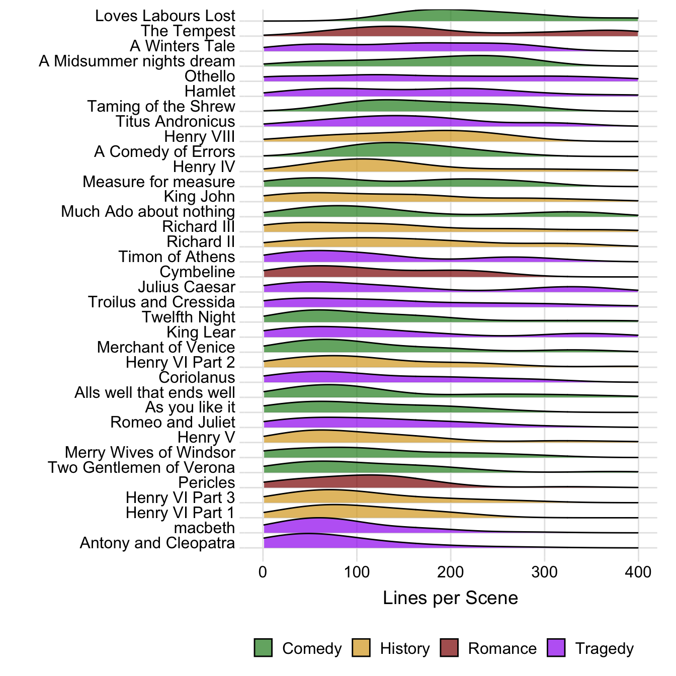
Sunday, 31 May 2026
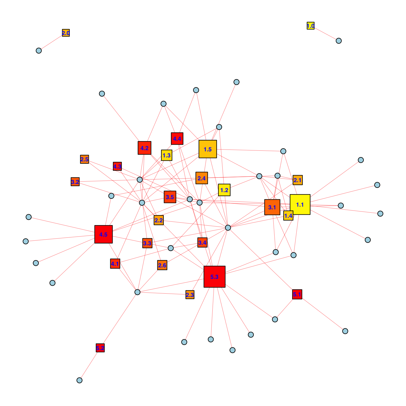
William Shakespeare’s plays are a continual source of fascination and delight. They also contain all sorts of features intriguing from digital humanities and data science perspectives. For a bit of fun and with very little explanation so far, below are visualisations of Shakespeare’s plays, most especially as network graphs.
# A tibble: 4 × 2
Play_Genre Mean_Scene_Length
<chr> <dbl>
1 Comedy 151.
2 History 136.
3 Romance 147.
4 Tragedy 140.The dataset contains 105,153 lines of speech that make up Shakespeare’s plays. Figure 2 shows spread of plays by their total word count and total number of speeches (as others have shown).
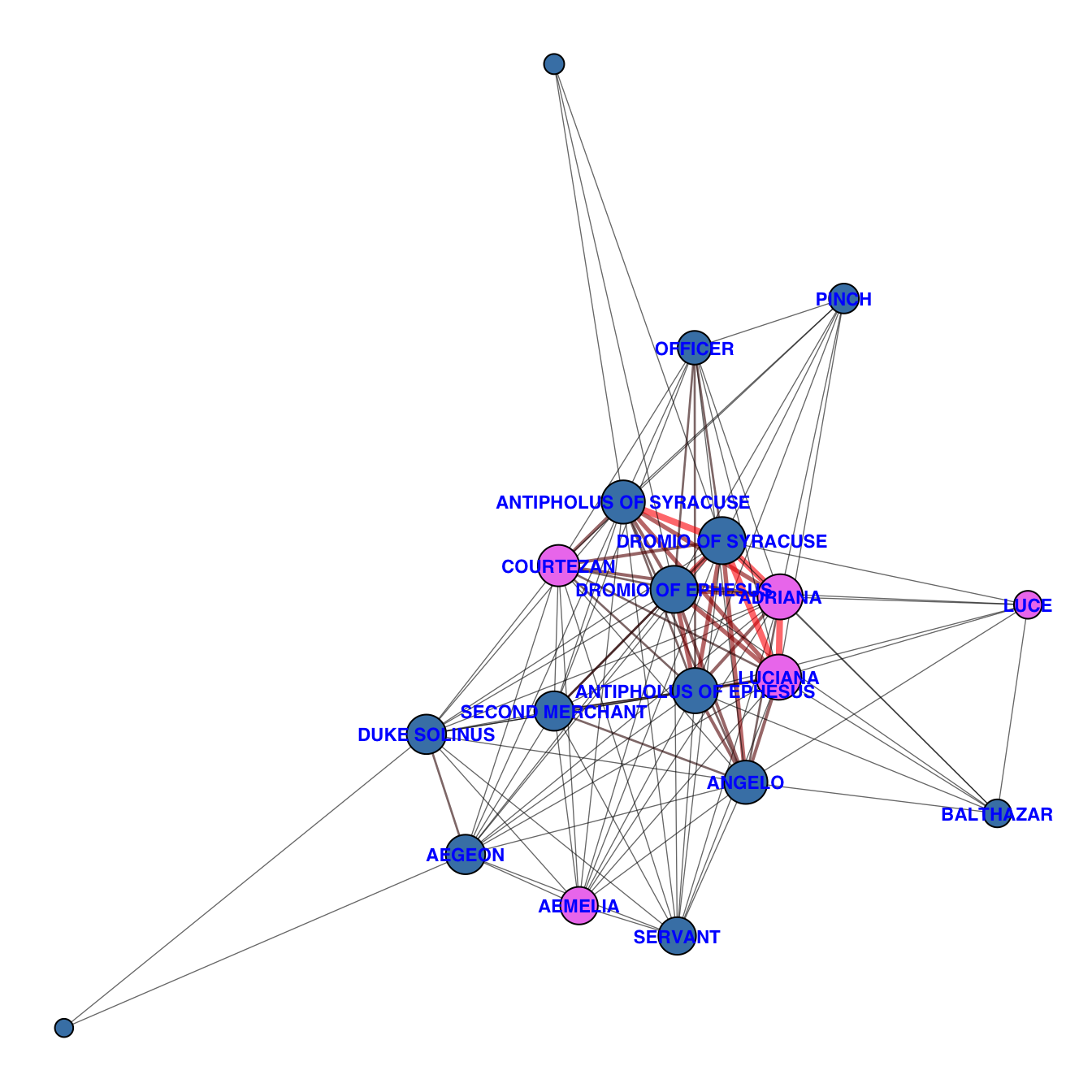
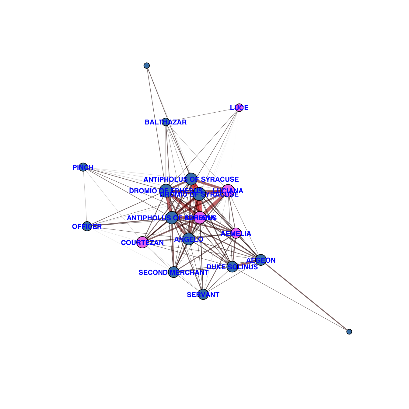
Set in the Greek city of Ephesus, The Comedy of Errors tells the story of two sets of identical twins who were accidentally separated at birth. Antipholus of Syracuse and his servant, Dromio of Syracuse, arrive in Ephesus, which turns out to be the home of their twin brothers, Antipholus of Ephesus and his servant, Dromio of Ephesus. When the Syracusans encounter the friends and families of their twins, a series of wild mishaps based on mistaken identities lead to wrongful beatings, a near-seduction, the arrest of Antipholus of Ephesus, and false accusations of infidelity, theft, madness, and demonic possession.
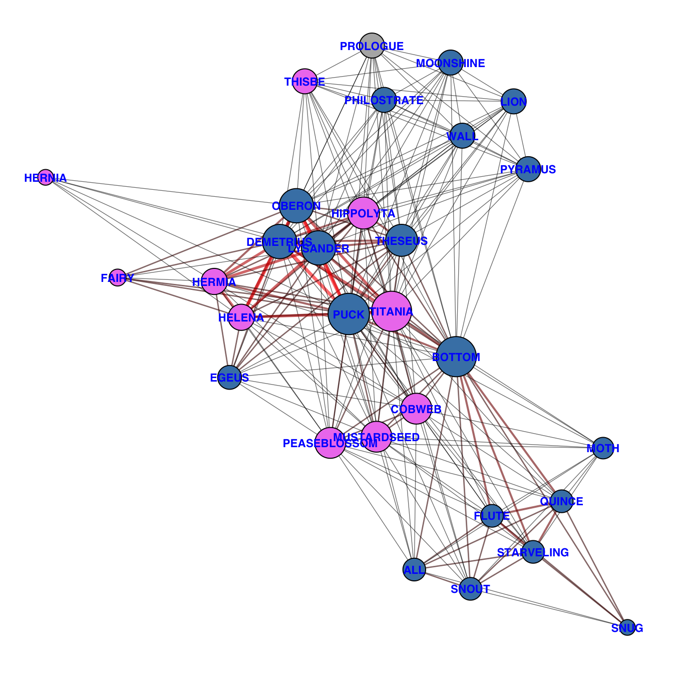
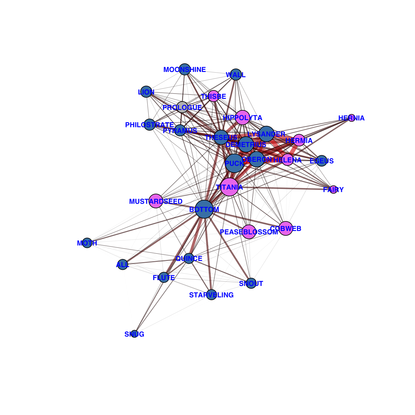
The play is set in Athens, and consists of several subplots that revolve around the marriage of Theseus and Hippolyta. One subplot involves a conflict among four Athenian lovers. Another follows a group of six amateur actors rehearsing the play which they are to perform before the wedding. Both groups find themselves in a forest inhabited by fairies who manipulate the humans and are engaged in their own domestic intrigue.
King Leontes’ jealousy leads him to wrongly accuse his wife of infidelity, causing tragedy. Years later, redemption, reconciliation, and miraculous reunions restore hope and family bonds.
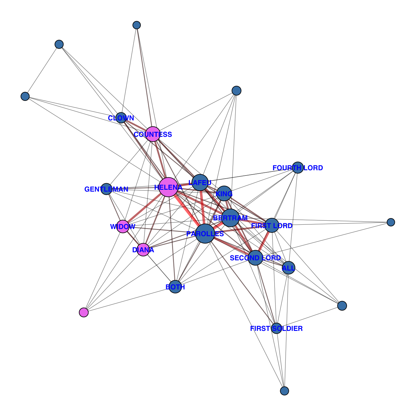
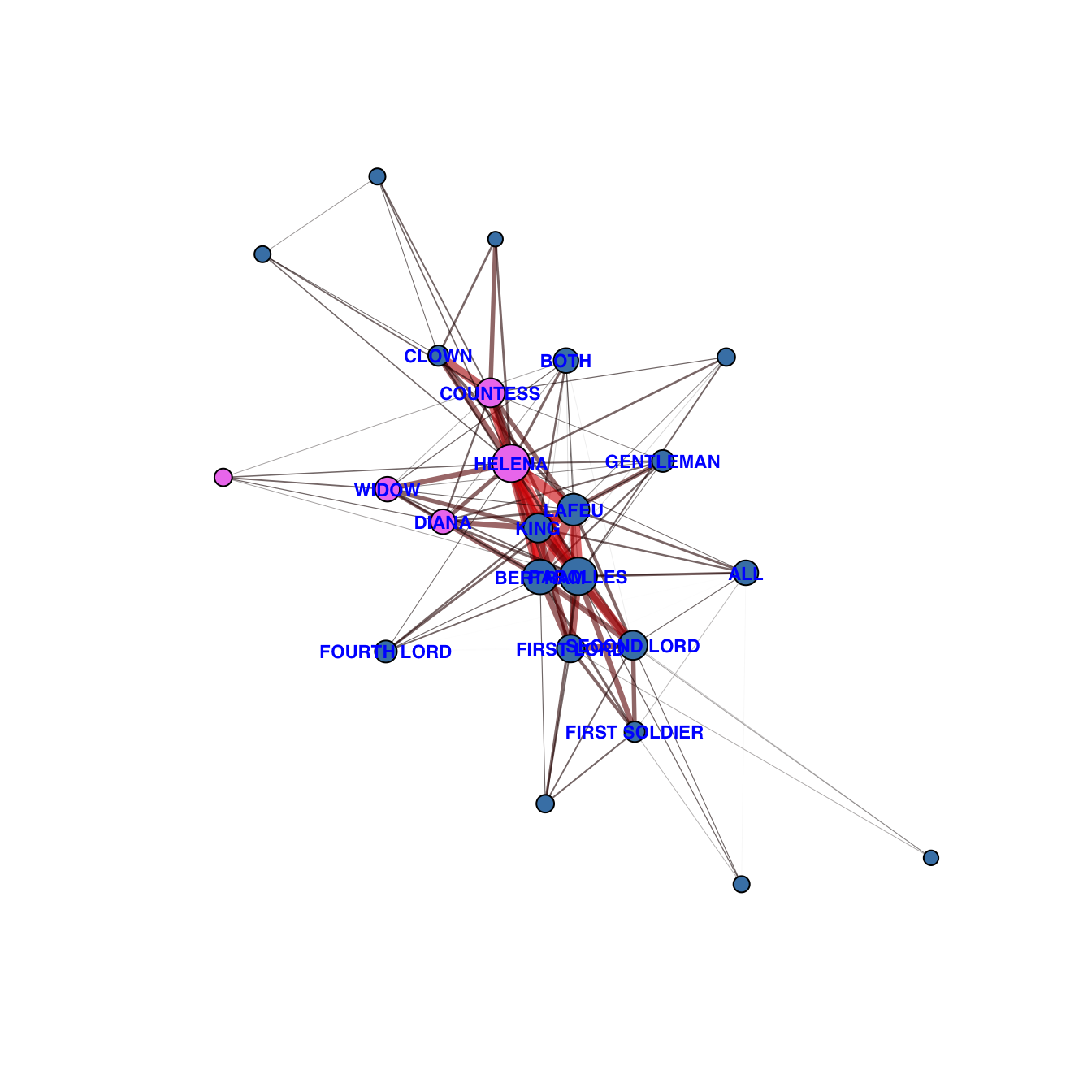
Helena cures the King of France’s illness and pursues her love, Bertram, through clever schemes. Challenges, misunderstandings, and social constraints are overcome, emphasizing perseverance and wit.
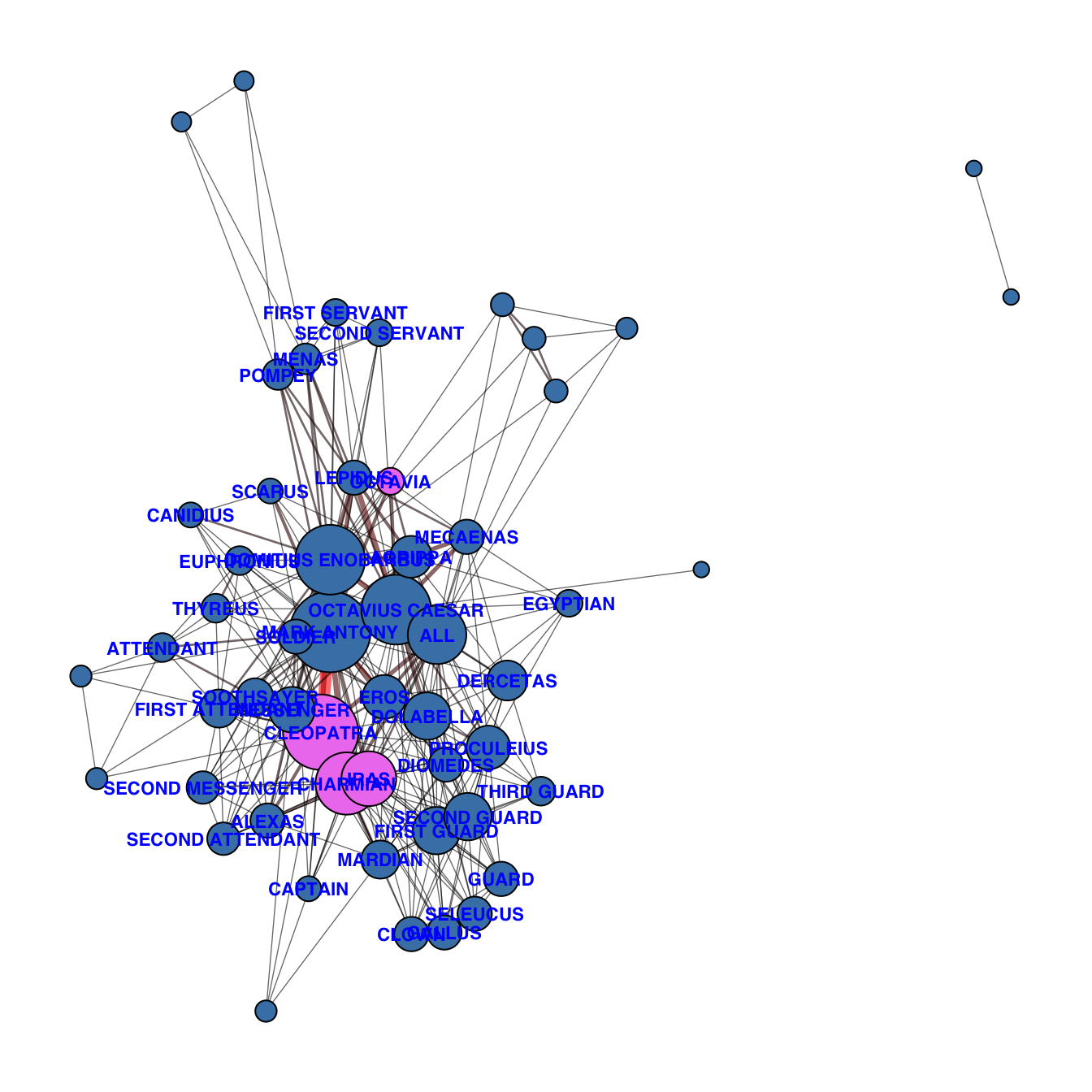
The plot is based on Thomas North’s 1579 English translation of Plutarch’s Lives (in Ancient Greek) and follows the relationship between Cleopatra and Mark Antony from the time of the Sicilian revolt to Cleopatra’s suicide during the War of Actium. The main antagonist is Octavius Caesar, one of Antony’s fellow triumvirs of the Second Triumvirate and the first emperor of the Roman Empire. The tragedy is mainly set in the Roman Republic and Ptolemaic Egypt and is characterized by swift shifts in geographical location and linguistic register as it alternates between sensual, imaginative Alexandria and a more pragmatic, austere Rome.
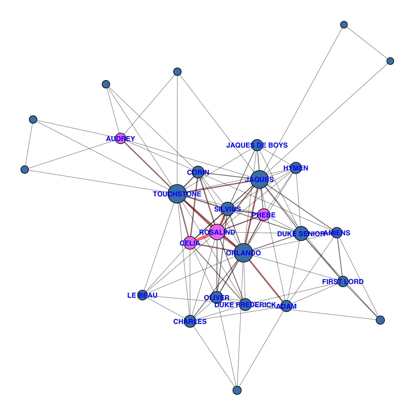
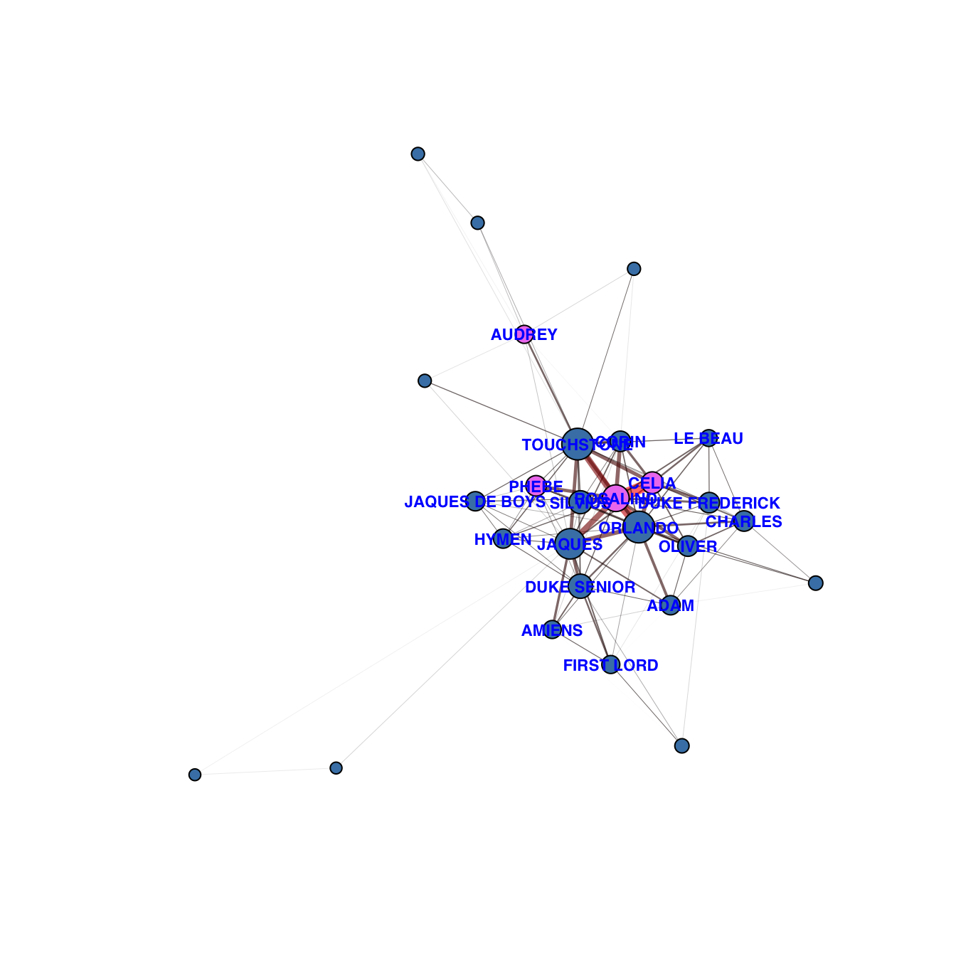
As You Like It follows its heroine Rosalind as she flees persecution in her uncle’s court, accompanied by her cousin Celia to find safety and, eventually, love, in the Forest of Arden. In the forest, they encounter a variety of memorable characters, notably the melancholy traveller Jaques, who speaks one of Shakespeare’s most famous speeches (“All the world’s a stage”) and provides a sharp contrast to the other characters in the play, always observing and disputing the hardships of life in the country.
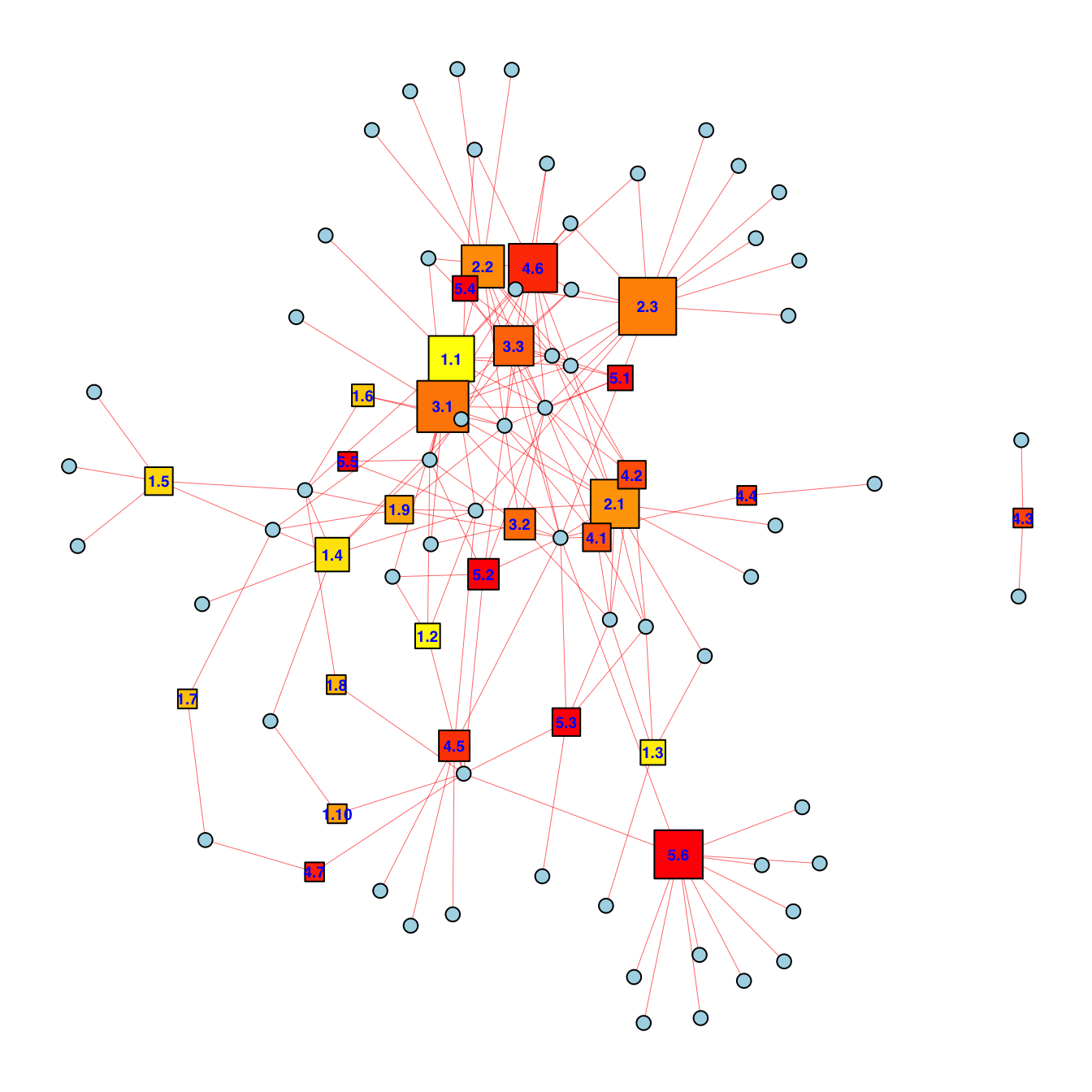
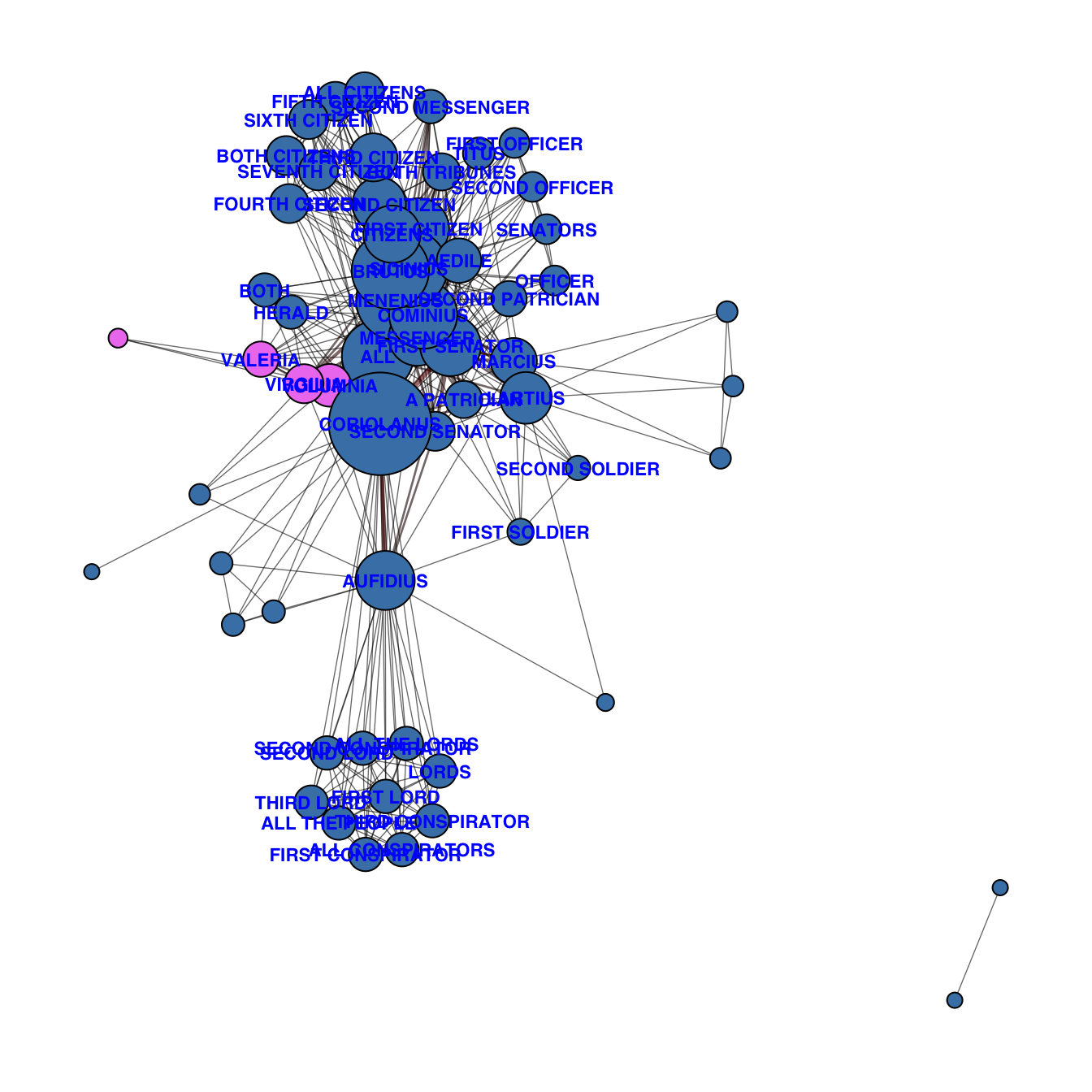
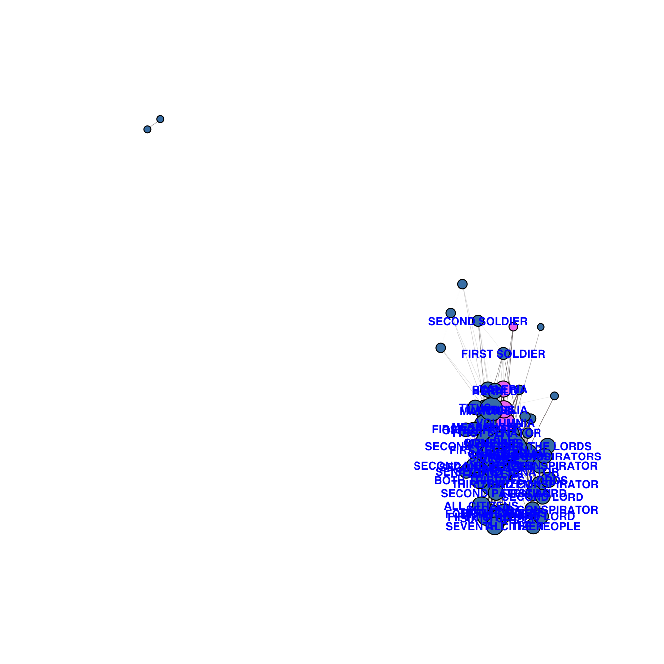
Coriolanus is the name given to a Roman general after his military feats against the Volscians at Corioli. Following his success, others encourage Coriolanus to pursue the consulship, but his disdain for the plebeians and mutual hostility with the tribunes lead to his banishment from Rome. In exile, he presents himself to the Volscians, then leads them against Rome. After he relents and agrees to a peace with Rome, he is killed by his previous Volscian allies.
Cymbeline, also known as The Tragedie of Cymbeline or Cymbeline, King of Britain, is a play by William Shakespeare set in Ancient Britain (c.10–14 AD) and based on legends that formed part of the Matter of Britain concerning the early historical Celtic British King Cunobeline.
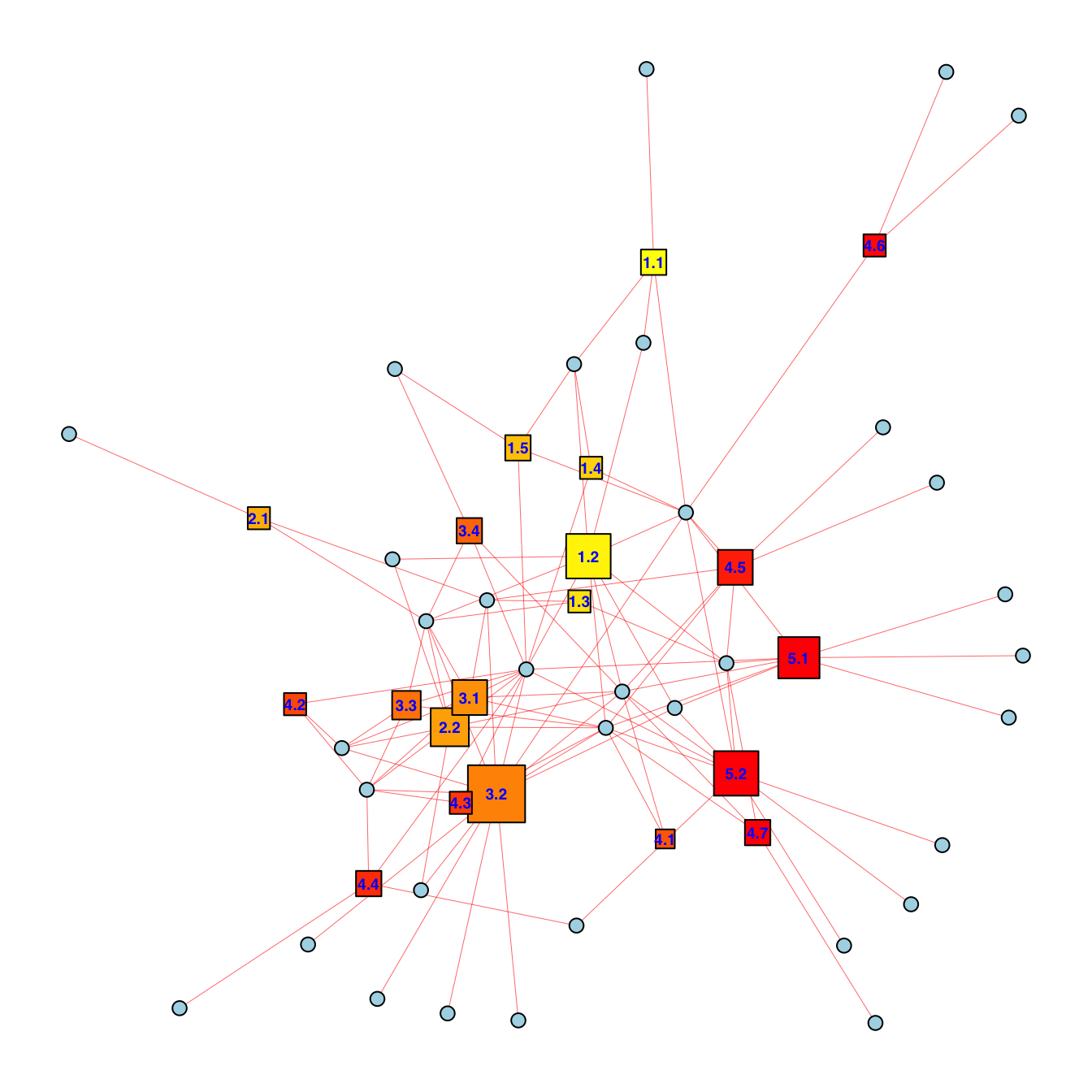
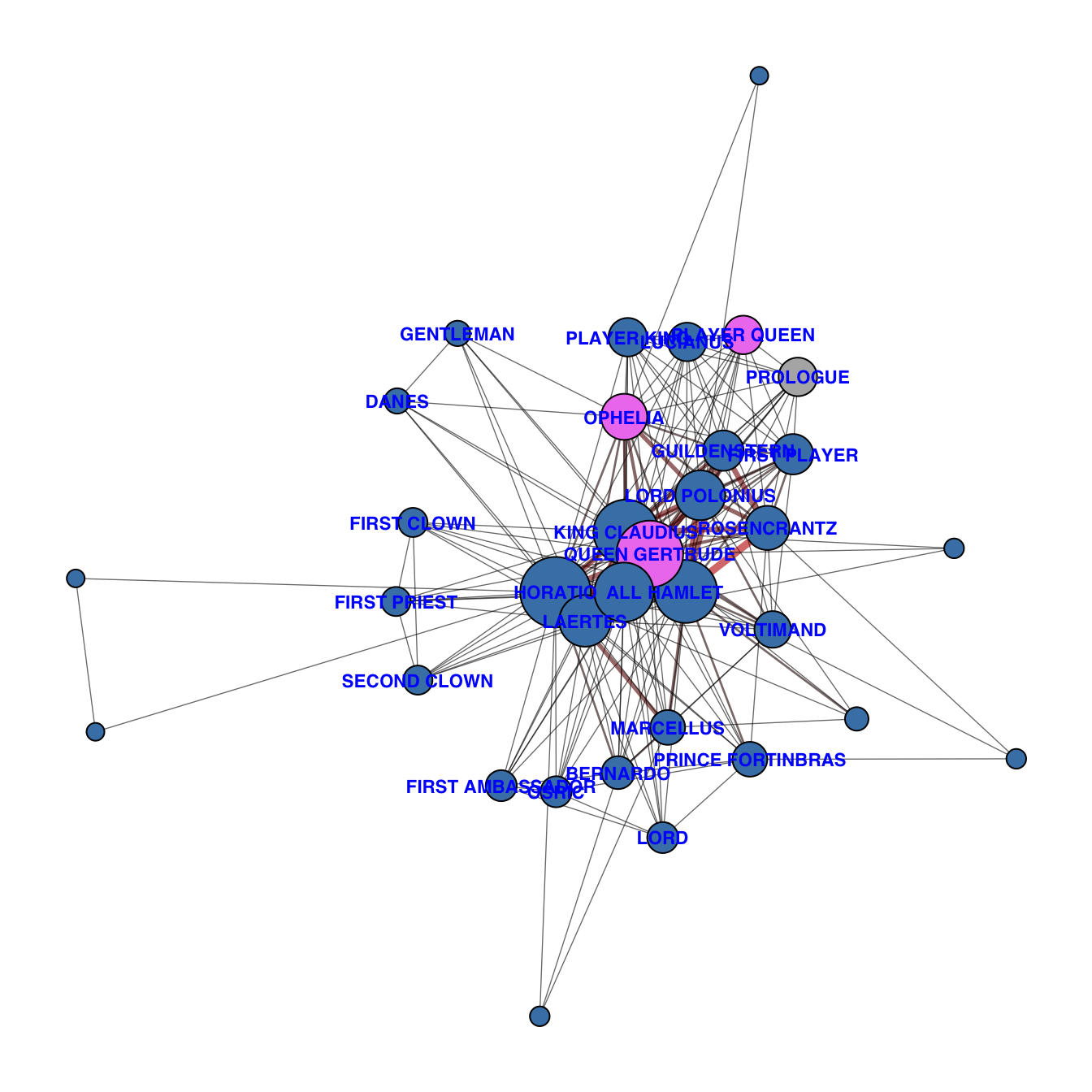
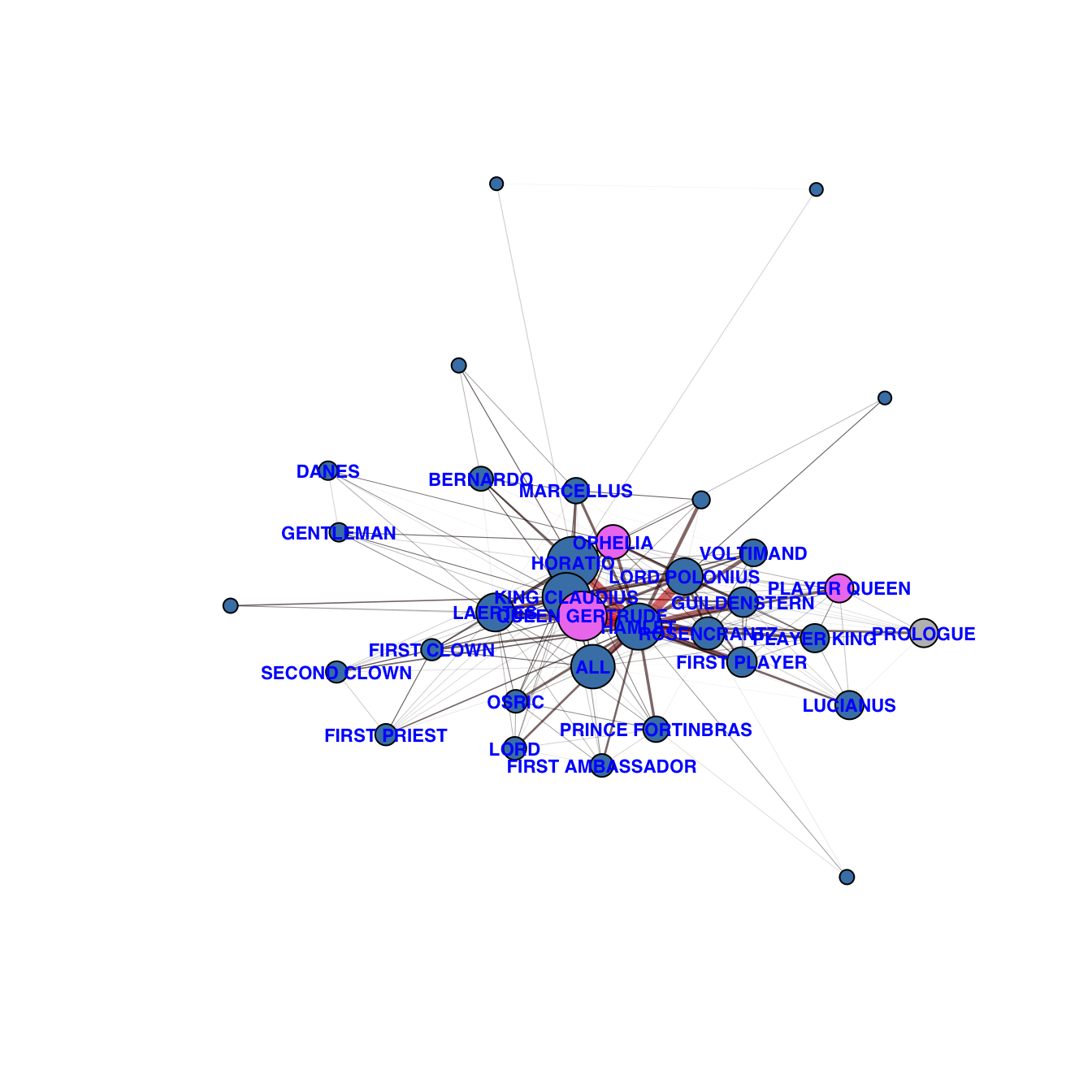
Set in Denmark, the play depicts Prince Hamlet and his attempts to exact revenge against his uncle, Claudius, who has murdered Hamlet’s father in order to seize his throne and marry Hamlet’s mother.
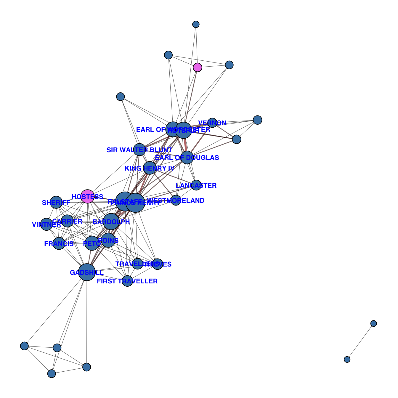
It was composed in the later years of the reign of Elizabeth I, when questions of succession and political stability were prominent. Set in England in the early 1400s during the reign of Henry IV, the play depicts rebellion against the crown alongside the development of Prince Hal, the future Henry V, and examines themes of leadership and the formation of the heir apparent.
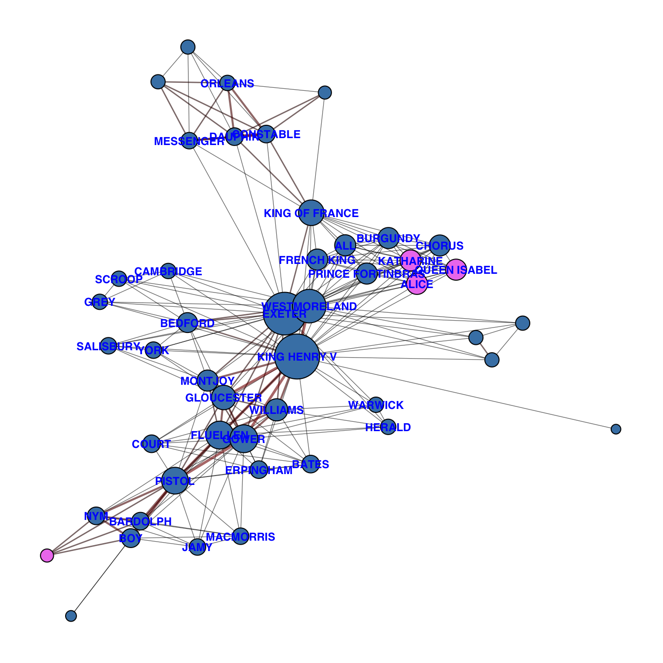
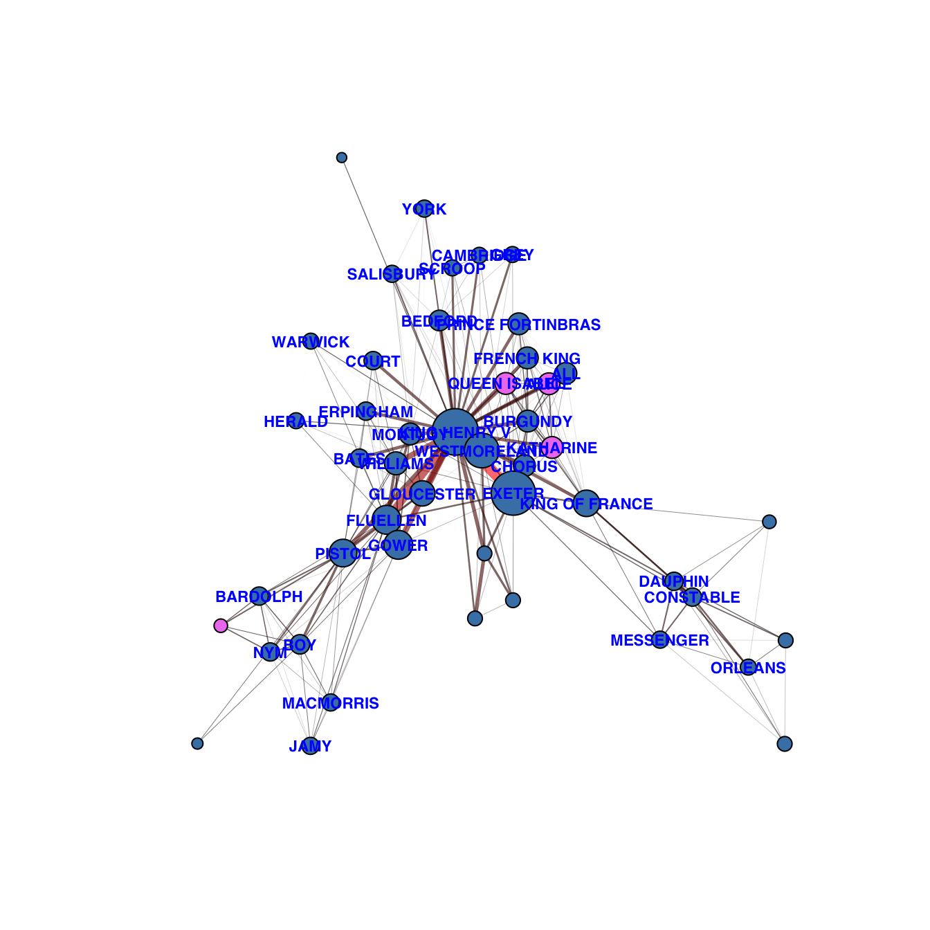
It tells the story of King Henry V of England, focusing on events immediately before and after the Battle of Agincourt (1415) during the Hundred Years’ War. In the First Quarto text, it was titled The Cronicle History of Henry the fift and The Life of Henry the Fifth in the First Folio text.
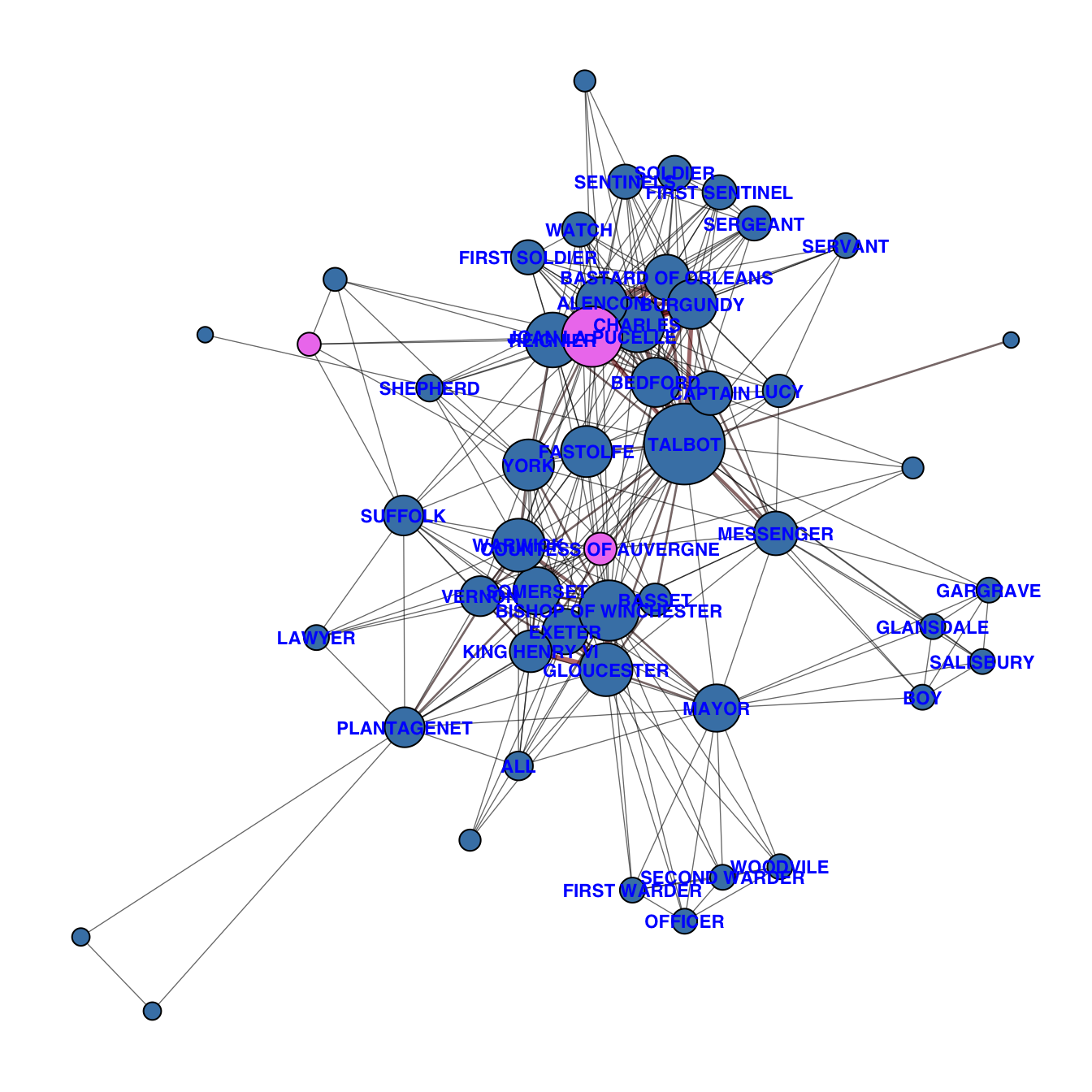
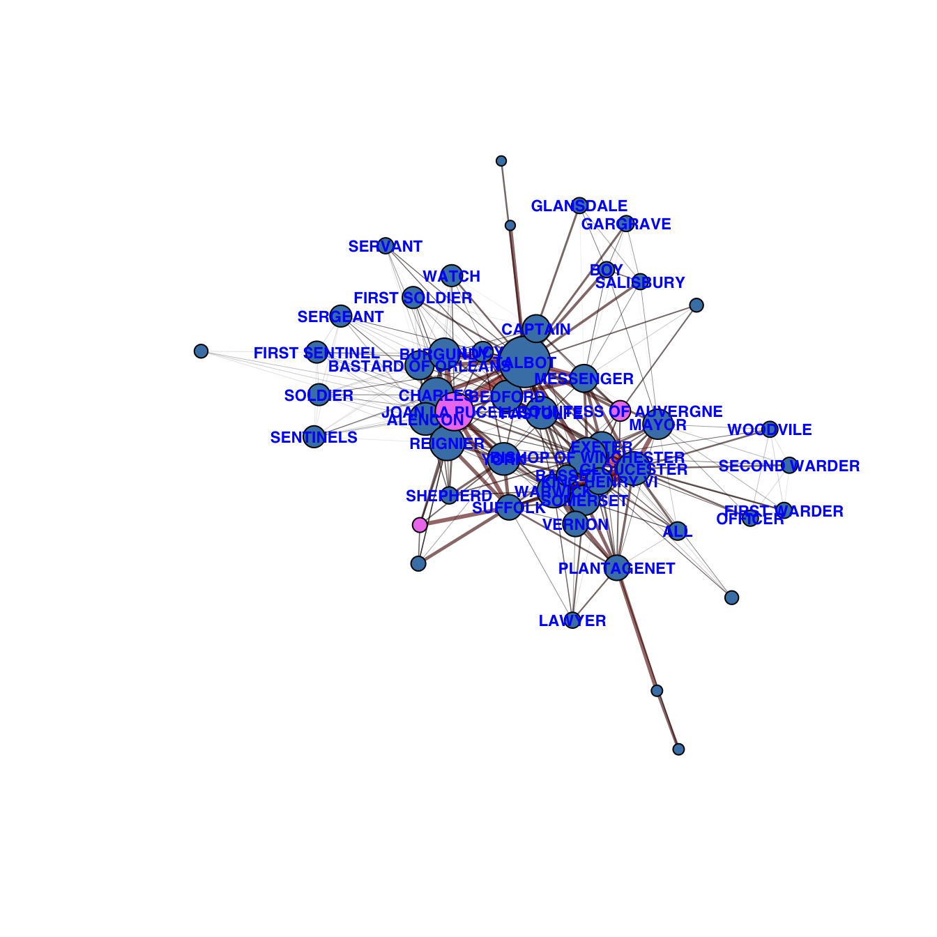
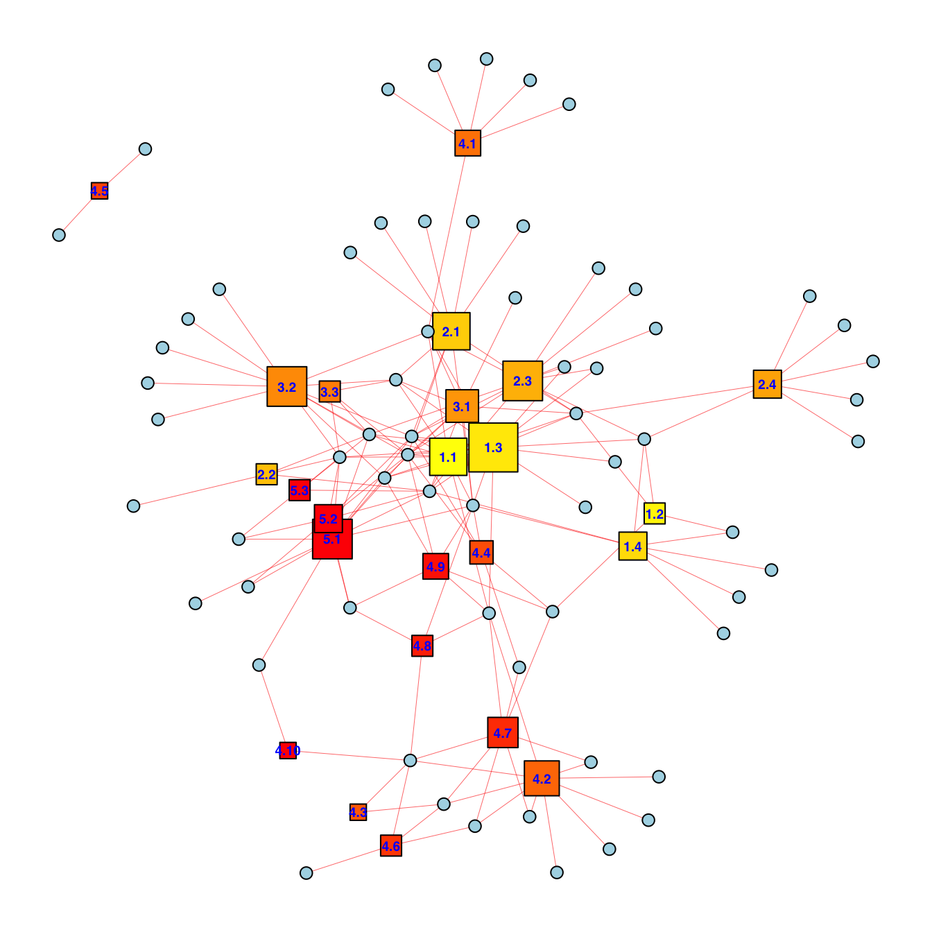
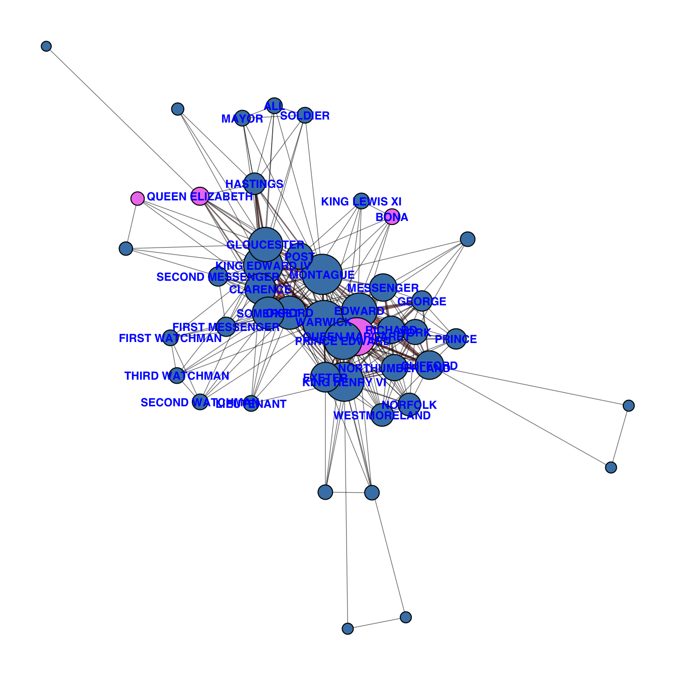
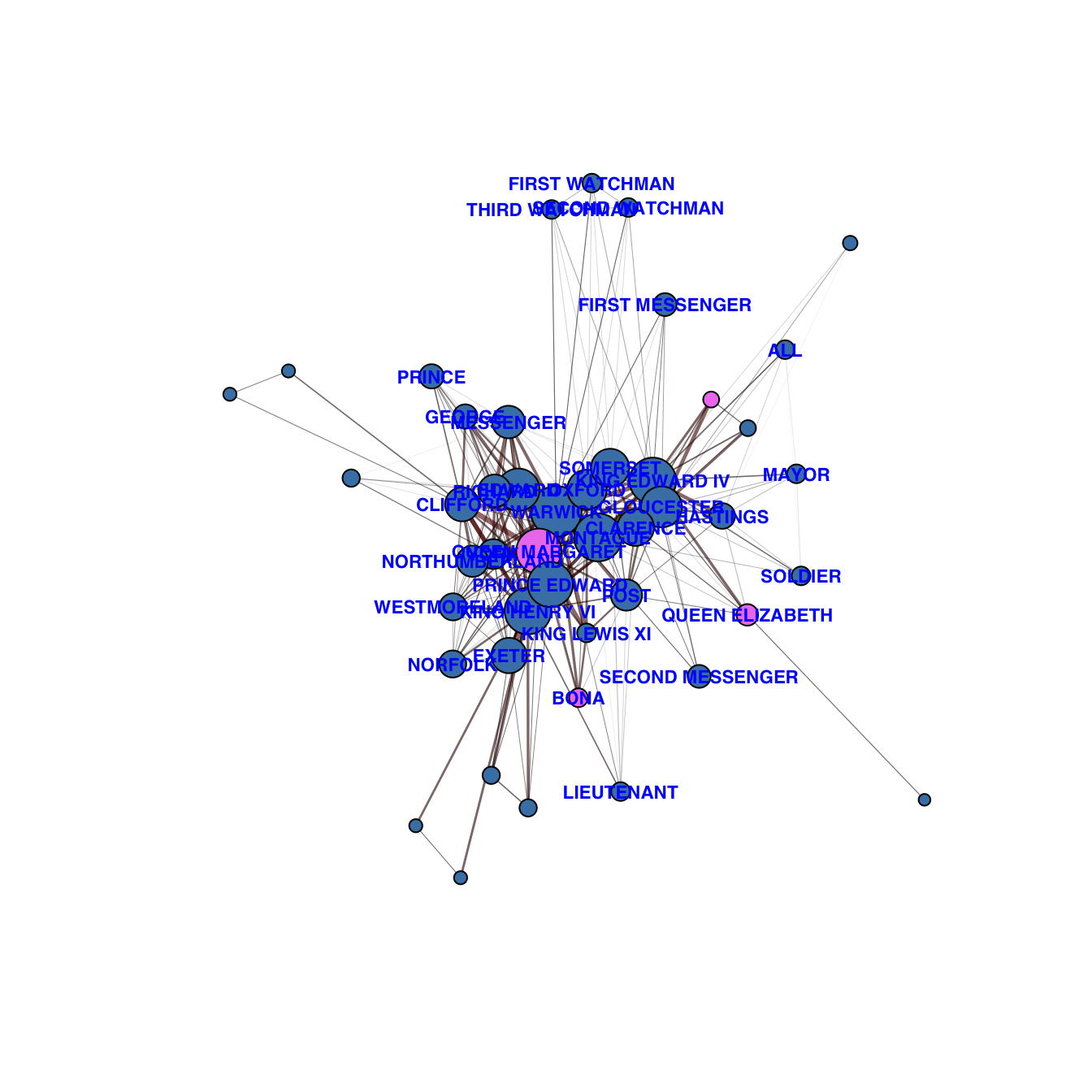
Henry VI, Part 1 deals with the loss of England’s French territories and the political machinations leading up to the Wars of the Roses, as the English political system is torn apart by personal squabbles and petty jealousy. Henry VI, Part 2 deals with the King’s inability to quell the bickering of his nobles and the inevitability of armed conflict and Henry VI, Part 3 deals with the horrors of that conflict.
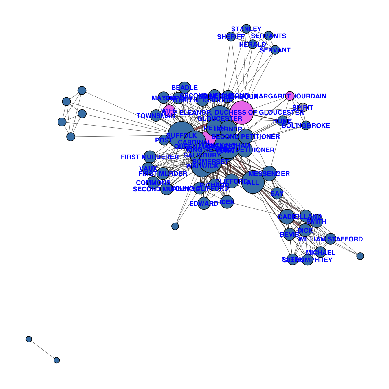
Henry VI, Part 2 (1591) is a Shakespearean history play about King Henry VI of England’s inability to quell the bickering of his noblemen, the death of his trusted advisor Humphrey, Duke of Gloucester, and the political rise of Richard of York, 3rd Duke of York; it culminates with the First Battle of St Albans (1455), the initial battle of the Wars of the Roses, which were civil wars between the House of Lancaster and the House of York.
Whereas 1 Henry VI deals with the loss of England’s French territories and the political machinations leading up to the Wars of the Roses and 2 Henry VI focuses on the King’s inability to quell the bickering of his nobles, and the inevitability of armed conflict, 3 Henry VI deals primarily with the horrors of that conflict, with the once stable nation thrown into chaos and barbarism as families break down and moral codes are subverted in the pursuit of revenge and power.
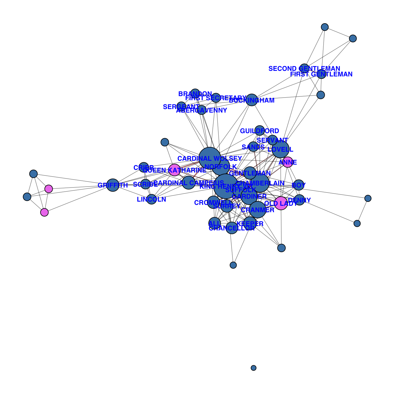
The Famous History of the Life of King Henry the Eighth, often shortened to Henry VIII, is a collaborative history play, written by William Shakespeare and John Fletcher, based on the life of Henry VIII. An alternative title, All Is True, is recorded in contemporary documents, with the title Henry VIII not appearing until the play’s publication in the First Folio of 1623.
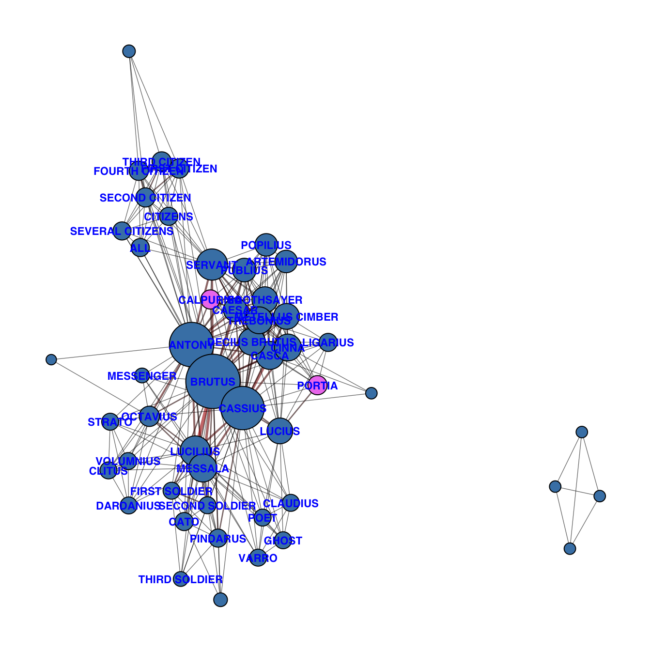
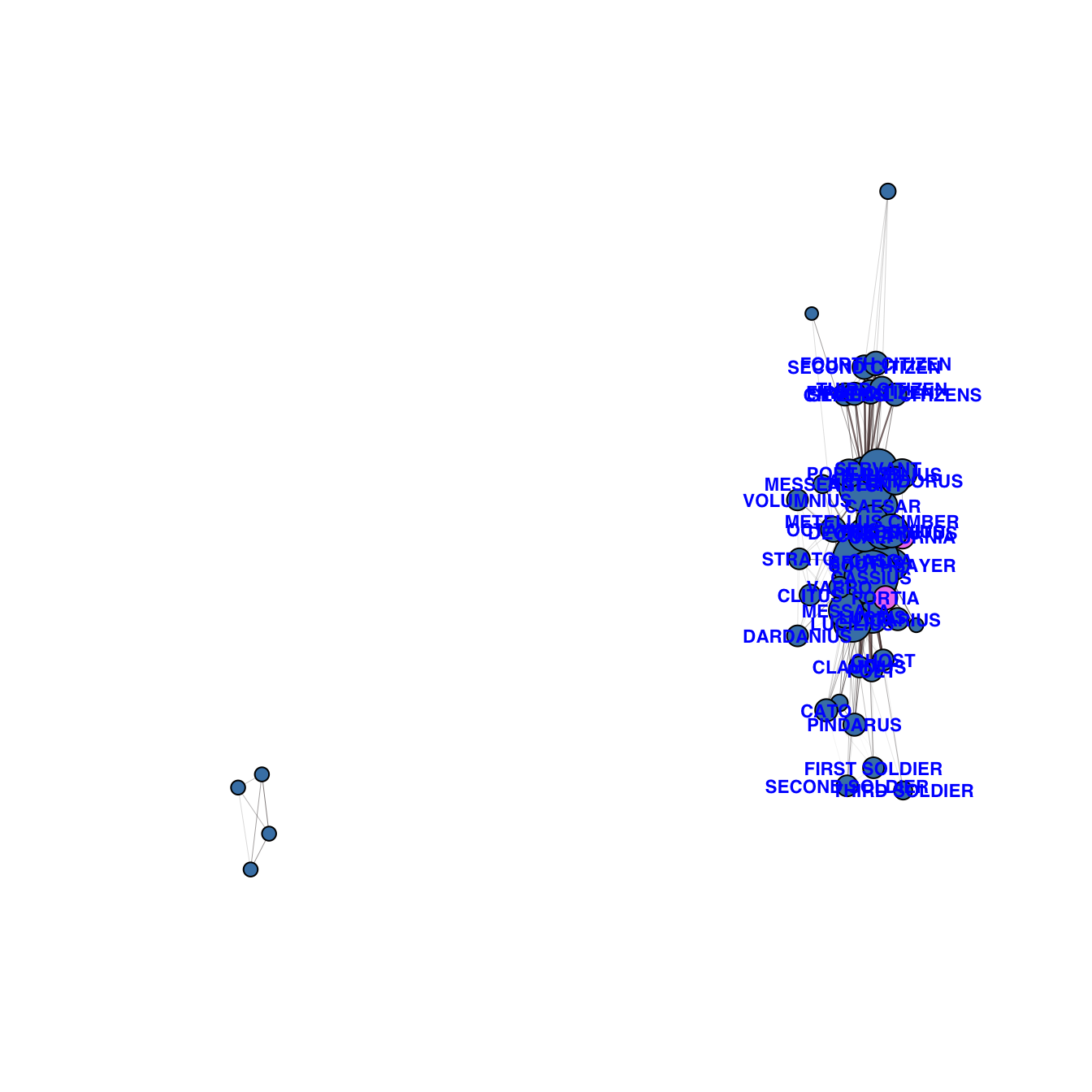
The play portrays the political conspiracy that led to the assassination of the Roman dictator Julius Caesar and Rome’s subsequent civil war. Drawing primarily (with deviations in various aspects) from Sir Thomas North’s 1579 translation of Parallel Lives by Plutarch, Shakespeare presents a dramatised account of Caesar’s growing power, his murder by a group of senators led by Cassius and Brutus, and the defeat of the conspirators by the forces of Mark Antony and Octavius at the Battle of Philippi.
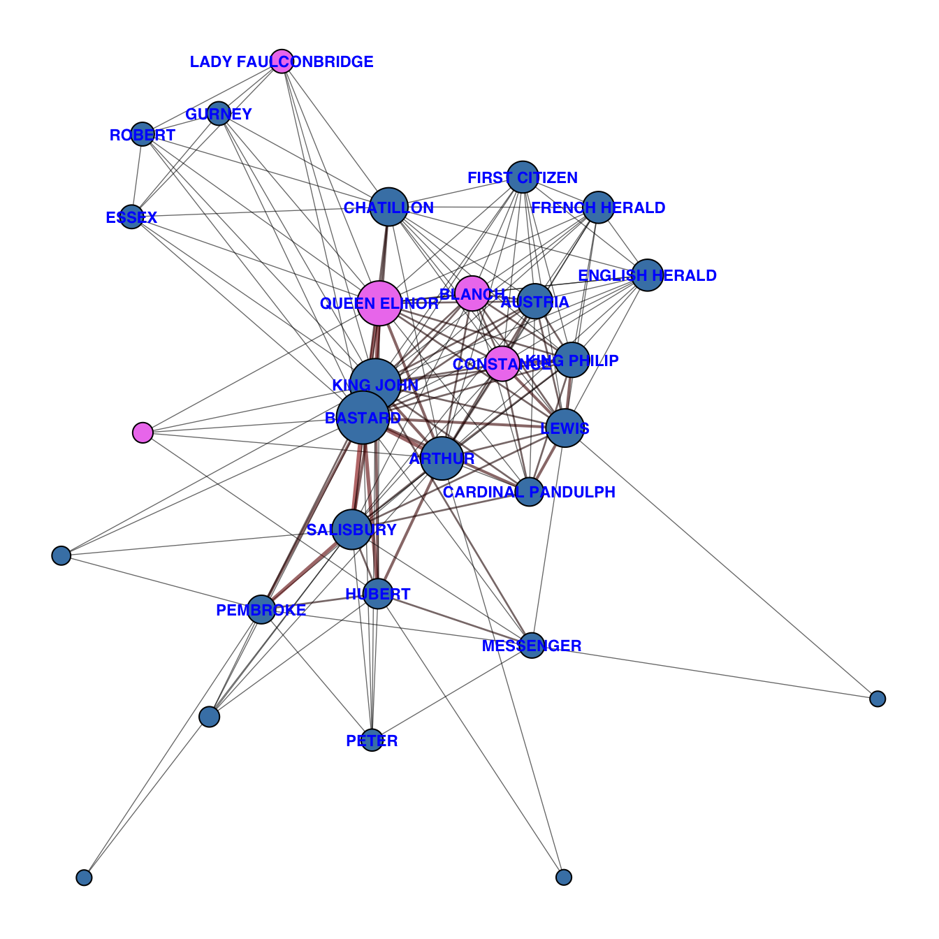
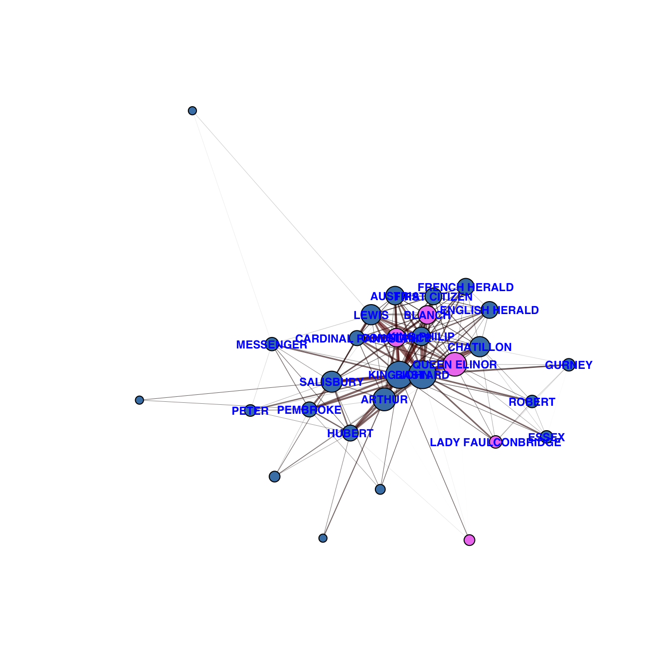
The Life and Death of King John (also King John) is a history play about the reign of John, King of England (r. 1199–1216), the son of Henry II and Eleanor of Aquitaine, and the father of Henry III.
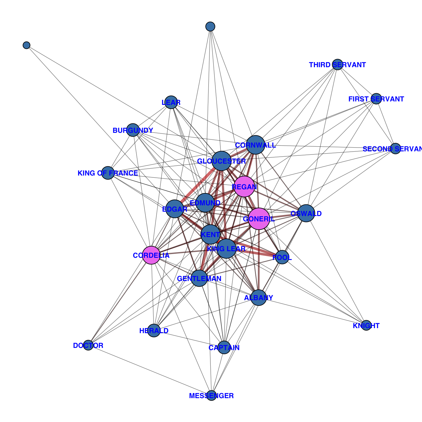
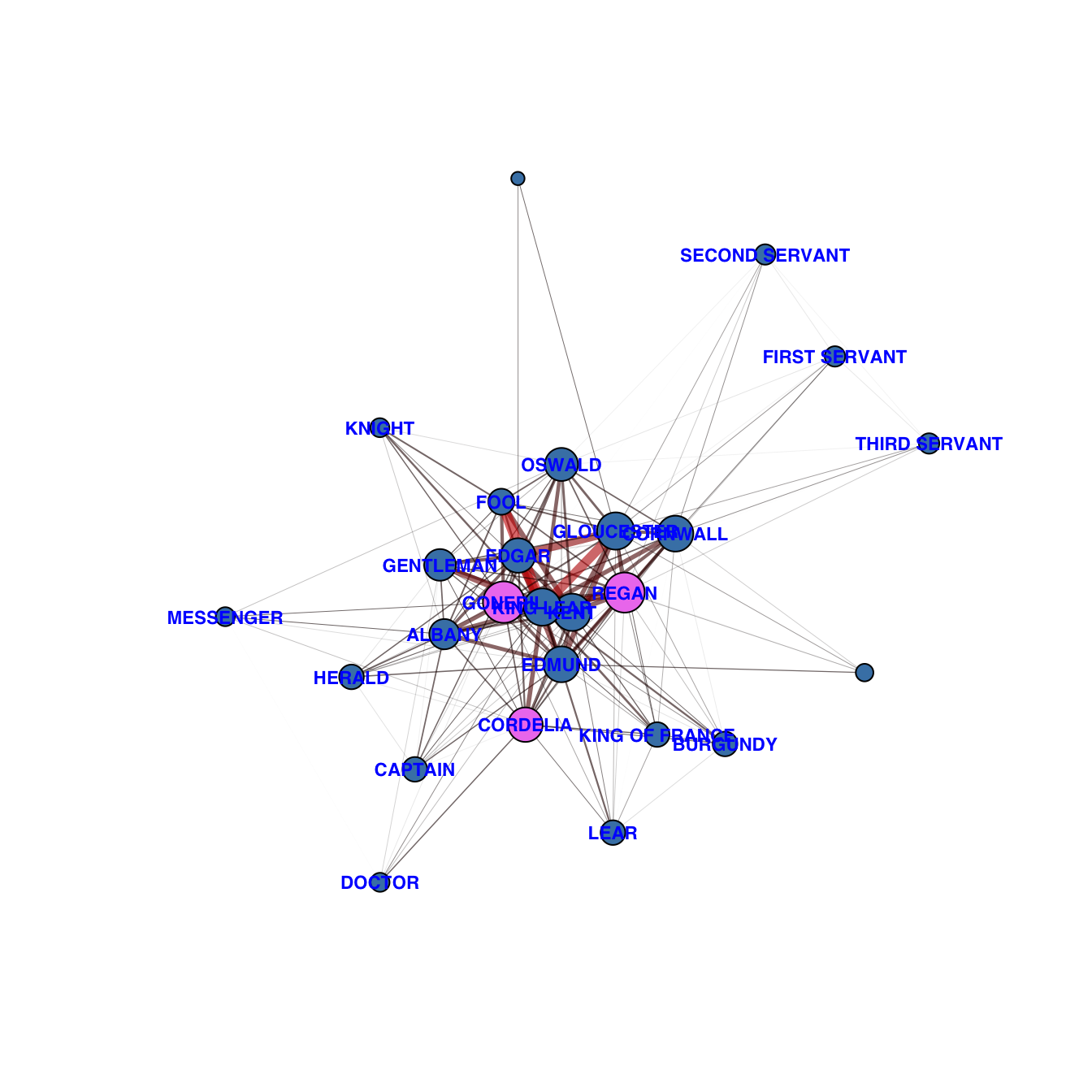
Set in pre-Roman Britain, the play depicts the consequences of King Lear’s love-test, in which he divides his power and land according to the praise of his daughters. The play is known for its dark tone, complex poetry, and prominent motifs concerning blindness, madness and human nature.
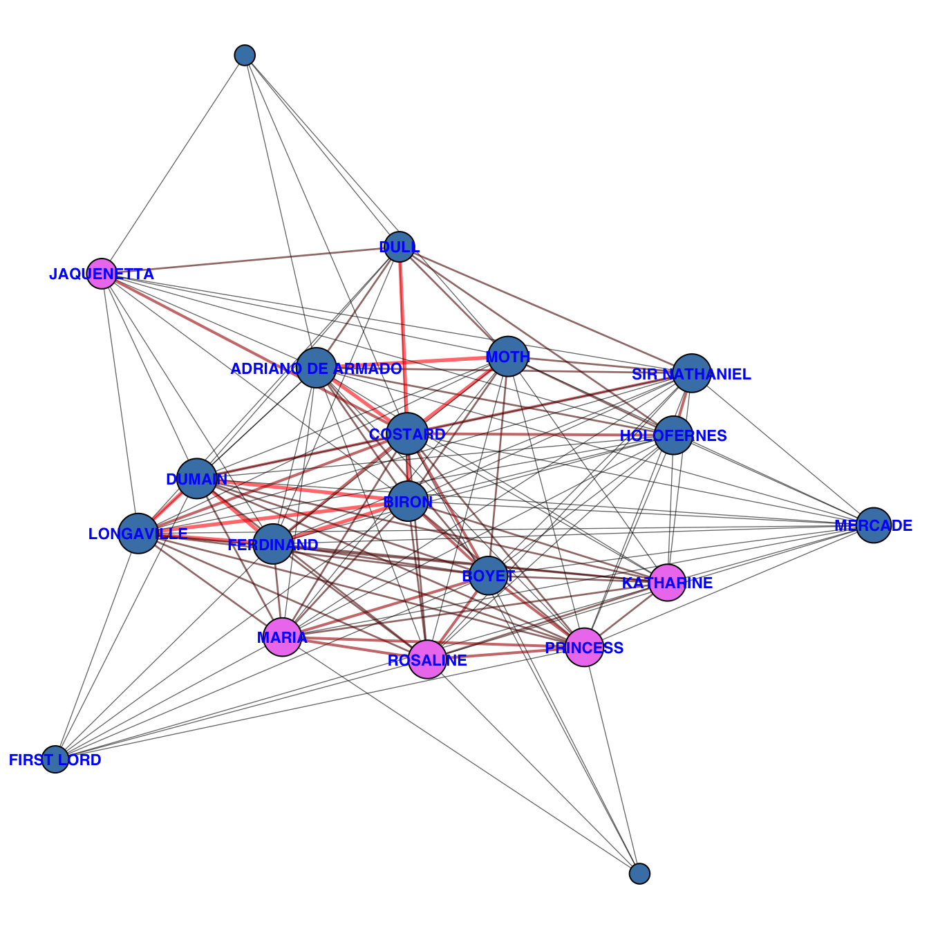
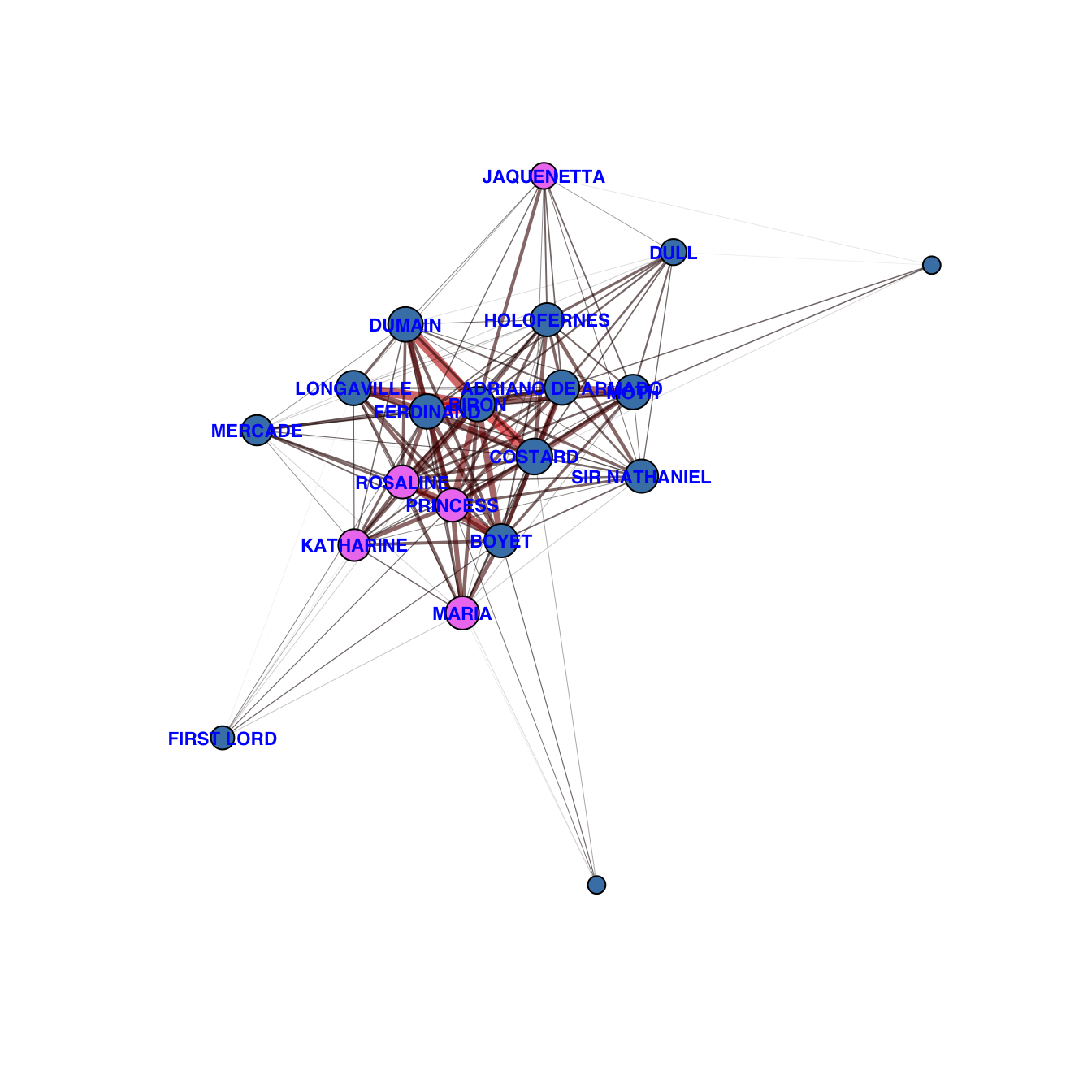
It follows the King of Navarre and his three companions as they attempt to swear off the company of women for three years in order to focus on study and fasting. Their subsequent infatuation with the Princess of France and her ladies makes them forsworn (break their oath). In an untraditional ending for a comedy, the play closes with the death of the Princess’s father, and all weddings are delayed for a year. The play draws on themes of masculine love and desire, reckoning and rationalisation, and reality versus fantasy.
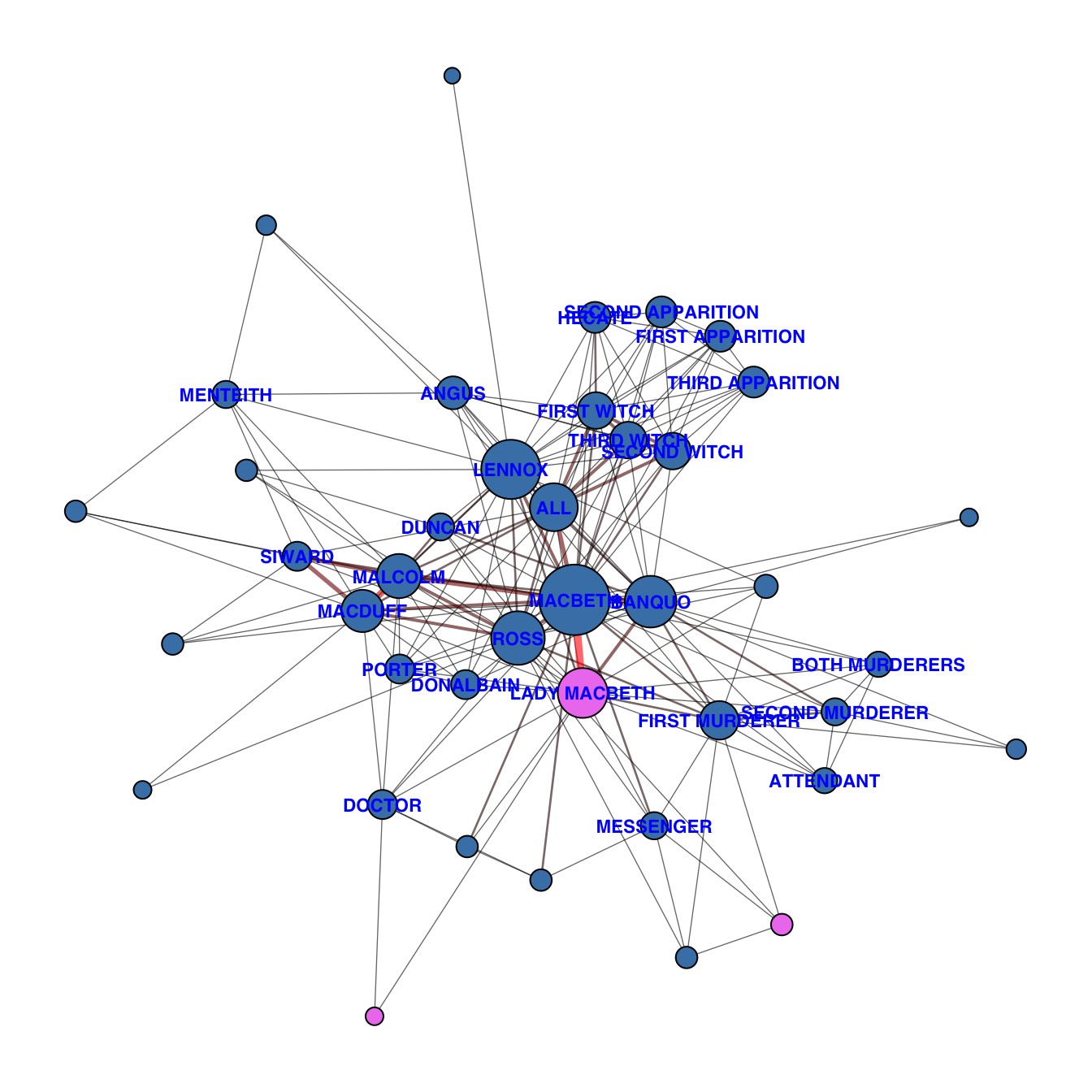
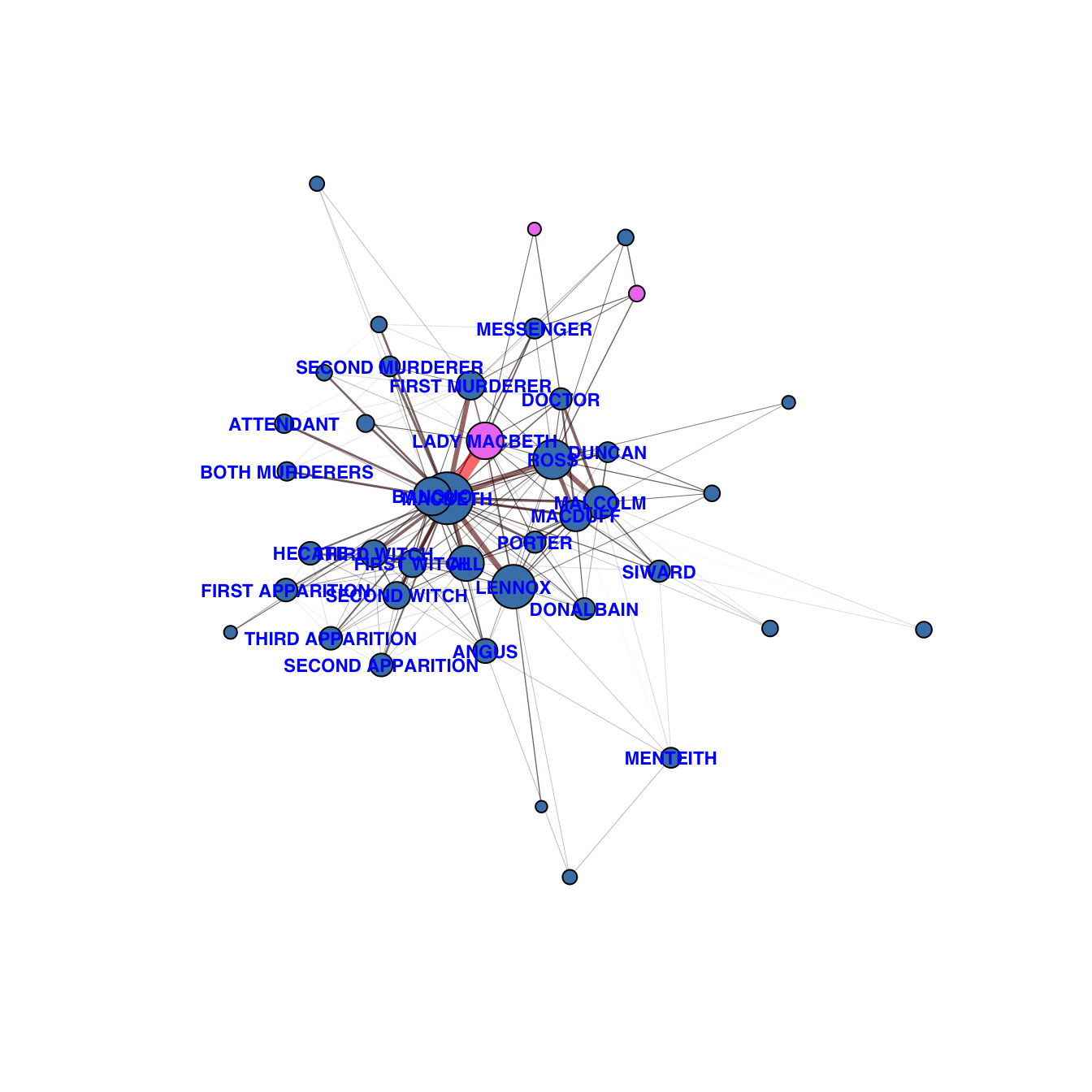
In the play, a brave Scottish general named Macbeth receives a prophecy from a trio of witches that one day he will become King of Scotland. Consumed by his latent ambition and spurred to violence by his wife, Macbeth murders King Duncan and takes the Scottish throne for himself. Then, racked with guilt and paranoia, he commits further murders to protect himself from enmity and suspicion, becoming a tyrannical ruler in the process. The violence perpetrated by the power-hungry couple leads to their insanity and finally to their deaths.
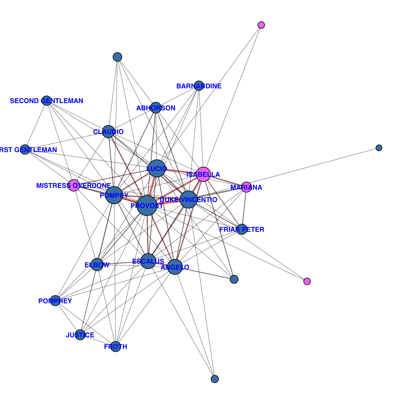
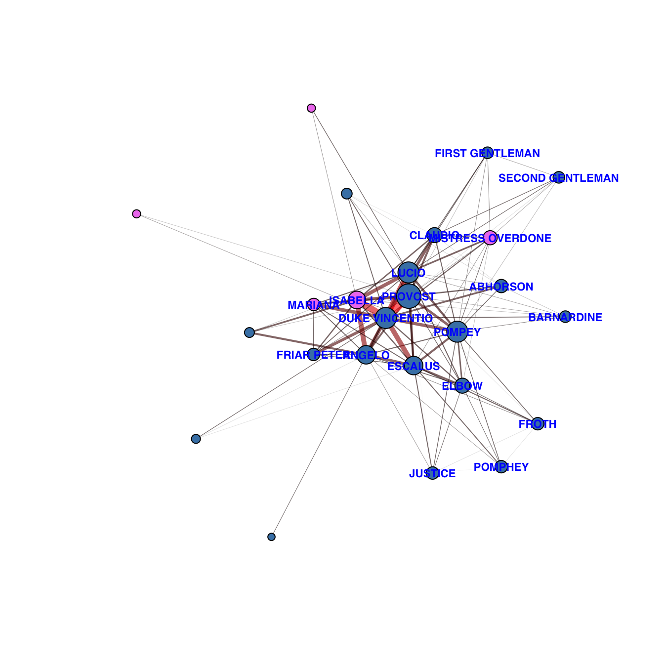
The play centres on the despotic and puritan Angelo, a deputy entrusted to rule the city of Vienna in the absence of Duke Vincentio, who instead disguises himself as a humble friar to observe Angelos regency and the lives of his citizens. Angelo persecutes a young man, Claudio, for the crime of fornication, sentencing him to death on a technicality. Angelo then attempts to exploit Isabella (the sister of Claudio), a chaste and innocent nun, when she comes to plead for the life of her brother.
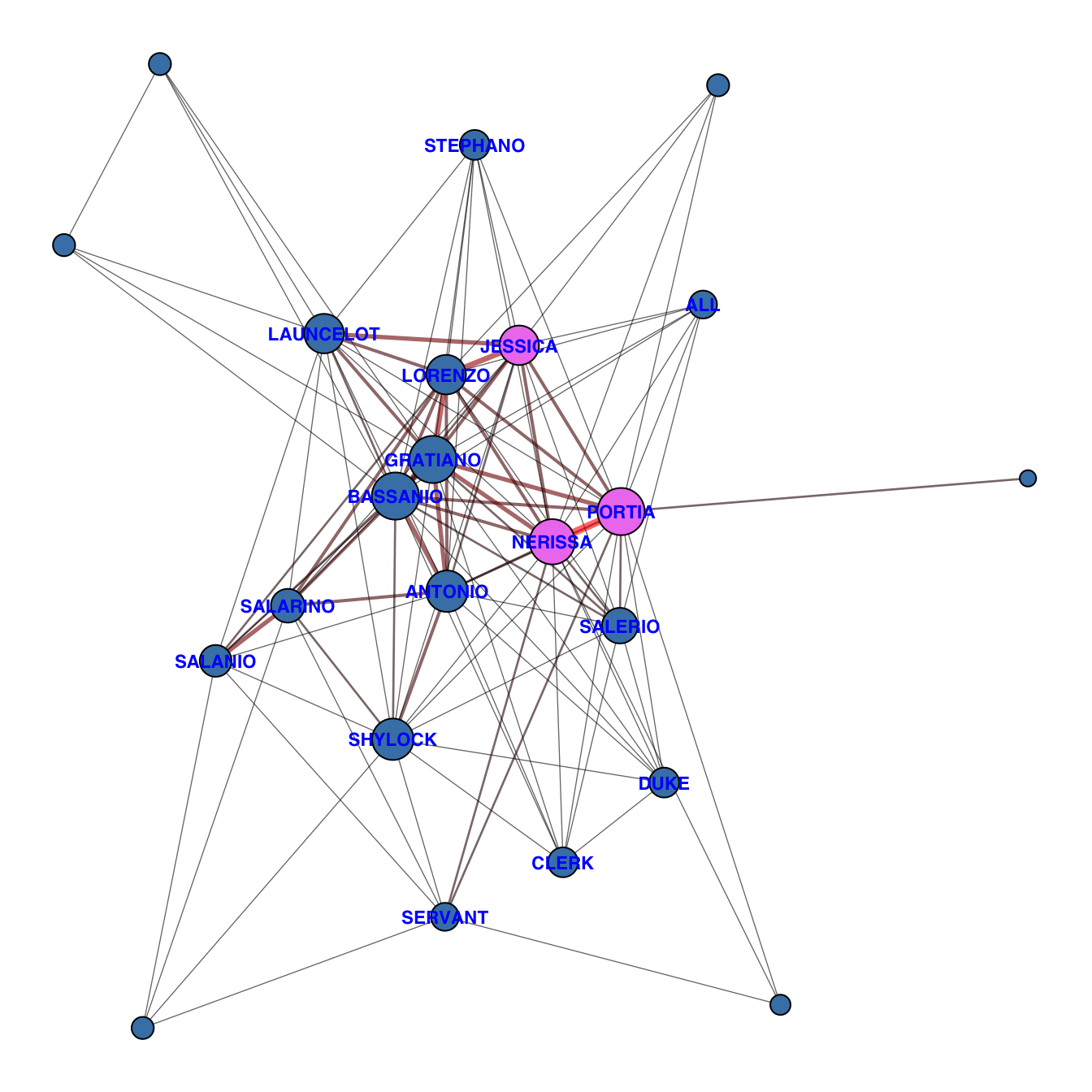
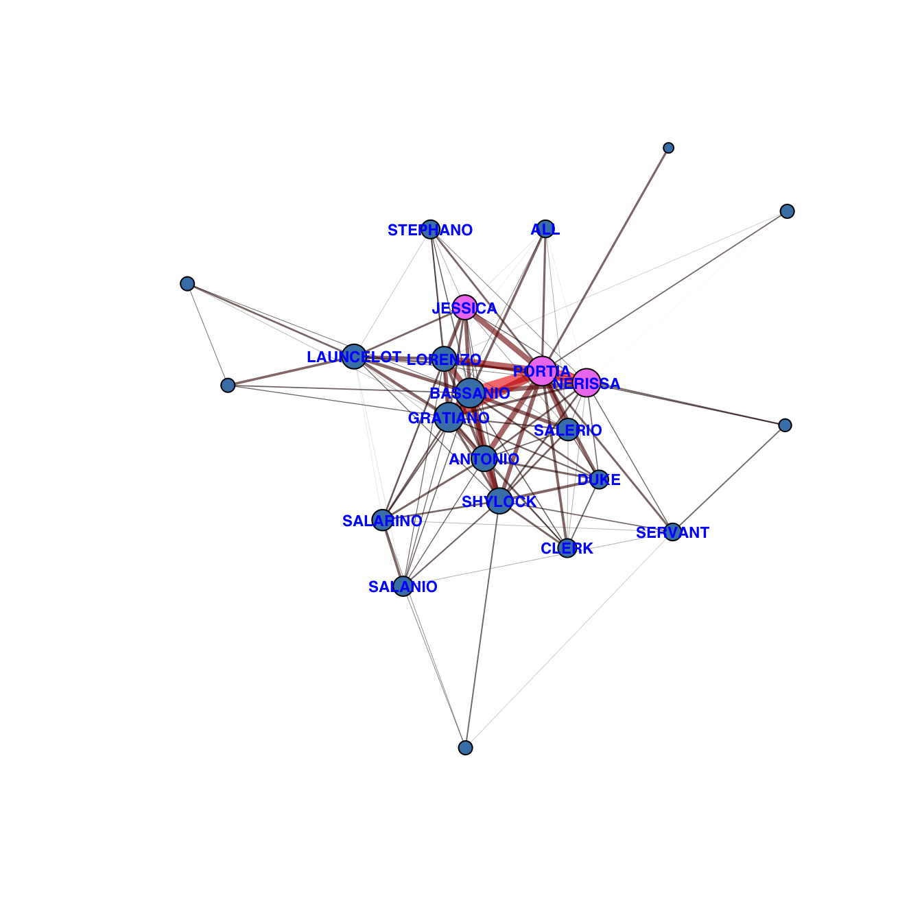
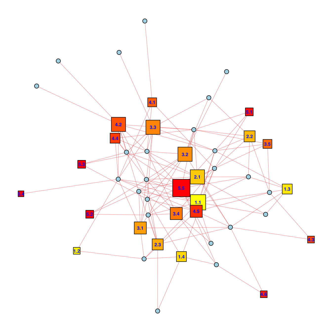
A merchant in Venice named Antonio defaults on a large loan taken out on behalf of his dear friend, Bassanio, and provided by a Jewish moneylender, Shylock, with seemingly inevitable fatal consequences.
SHYLOCK
Signior Antonio, many a time and oft
In the Rialto you have rated me
About my moneys and my usances:
Still have I borne it with a patient shrug,
For sufferance is the badge of all our tribe.
You call me misbeliever, cut-throat dog,
And spit upon my Jewish gaberdine,
And all for use of that which is mine own.
Well then, it now appears you need my help:
Go to, then, you come to me, and you say
'Shylock, we would have moneys:' you say so,
You, that did void your rheum upon my beard
And foot me as you spurn a stranger cur
Over your threshold: moneys is your suit
What should I say to you? Should I not say
'Hath a dog money? is it possible
A cur can lend three thousand ducats?' Or
Shall I bend low and in a bondman's key,
With bated breath and whispering humbleness, Say this,
'Fair sir, you spit on me on Wednesday last,
You spurn'd me such a day, another time
You call'd me dog, and for these courtesies
I'll lend you thus much moneys'?
PORTIA
The quality of mercy is not strain'd,
It droppeth as the gentle rain from heaven
Upon the place beneath: it is twice blest,
It blesseth him that gives and him that takes:
'Tis mightiest in the mightiest: it becomes
The throned monarch better than his crown,
His sceptre shows the force of temporal power,
The attribute to awe and majesty,
Wherein doth sit the dread and fear of kings,
But mercy is above this sceptred sway,
It is enthroned in the hearts of kings,
It is an attribute to God himself,
And earthly power doth then show likest God's
When mercy seasons justice. Therefore, Jew,
Though justice be thy plea, consider this,
That, in the course of justice, none of us
Should see salvation: we do pray for mercy,
And that same prayer doth teach us all to render
The deeds of mercy. I have spoke thus much
To mitigate the justice of thy plea,
Which if thou follow, this strict court of Venice
Must needs give sentence 'gainst the merchant there.
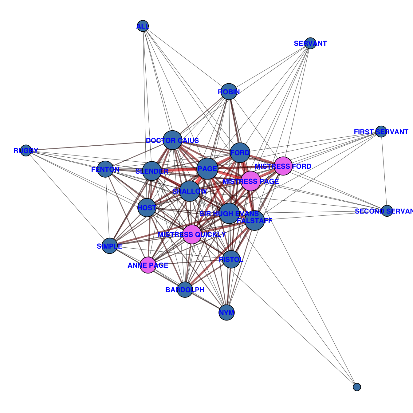
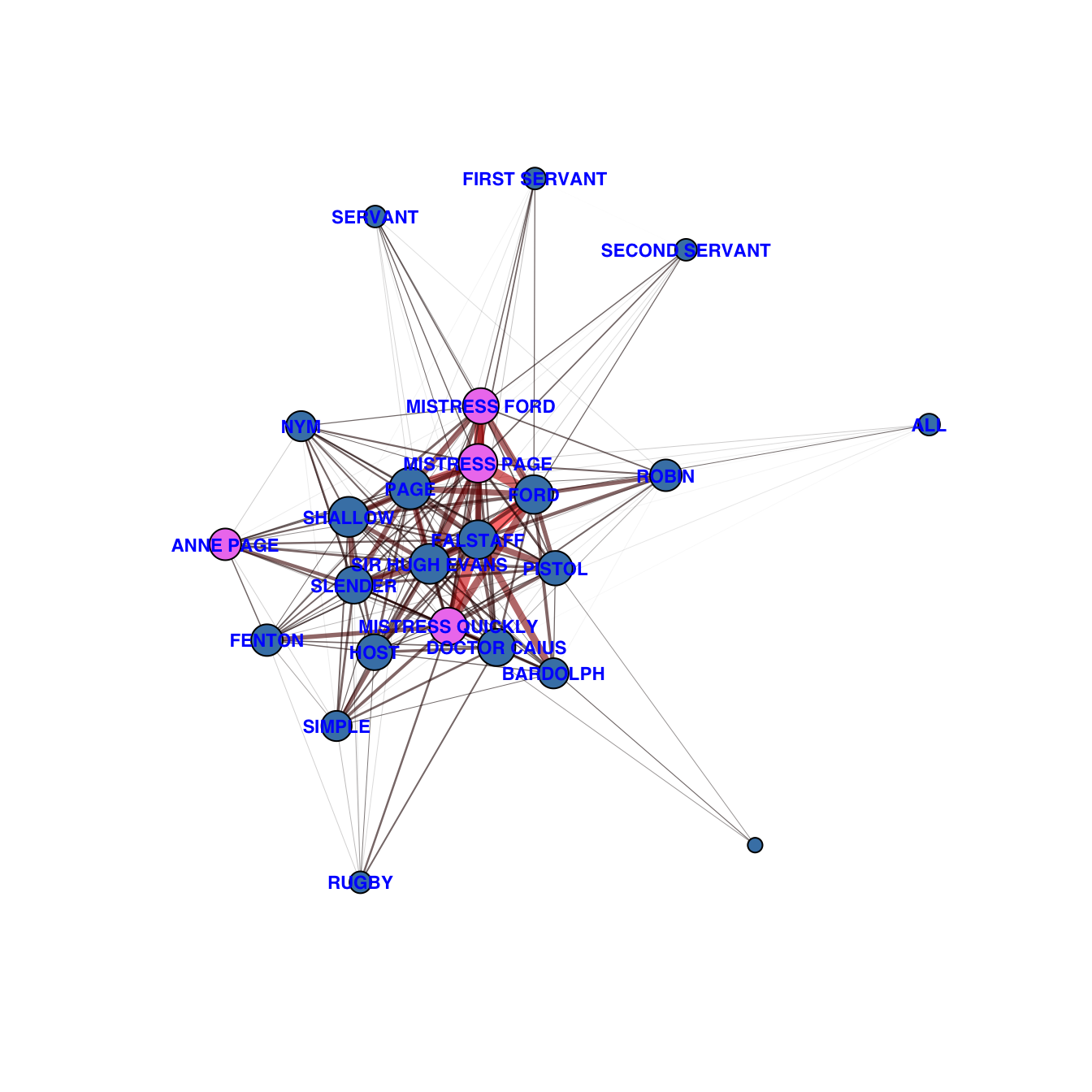
It features the character Sir John Falstaff, the fat knight who had previously been featured in Henry IV, Part 1 and Part 2. Tradition has it that The Merry Wives of Windsor was written at the request of Queen Elizabeth I, who watching Henry IV, Part 1, is said to have asked Shakespeare to write a play depicting Falstaff in love.
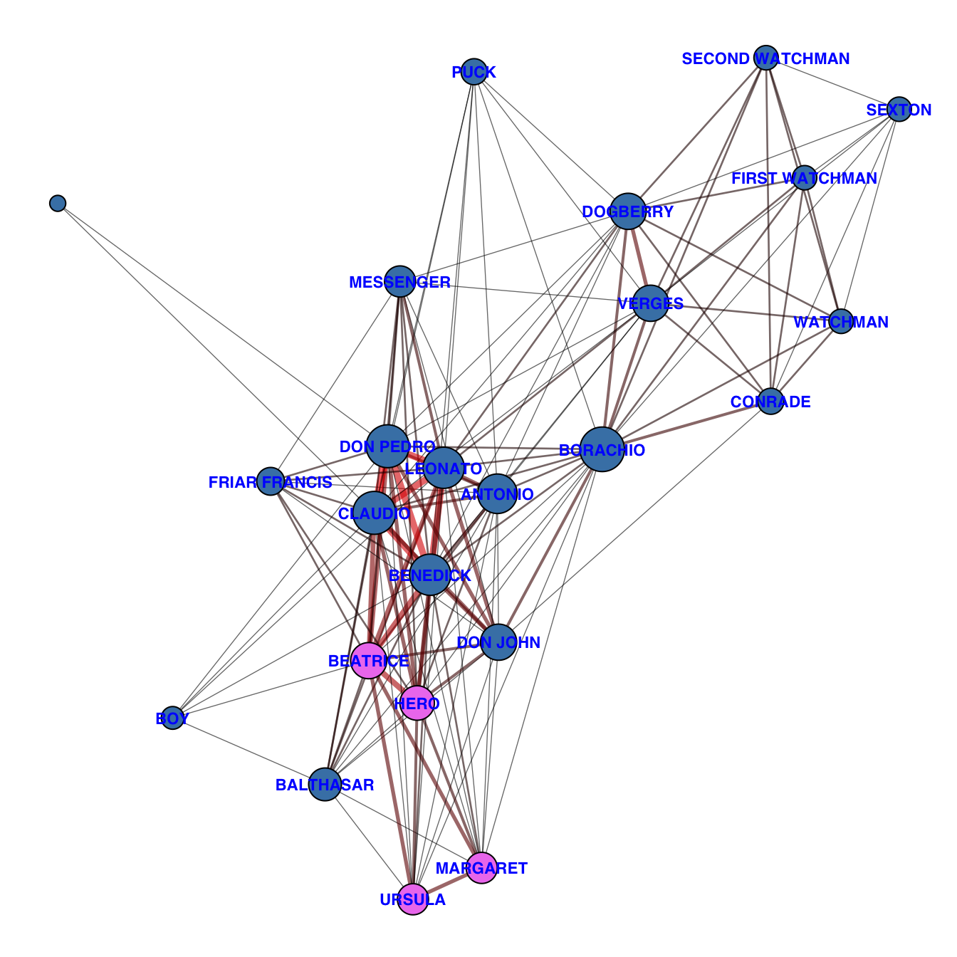
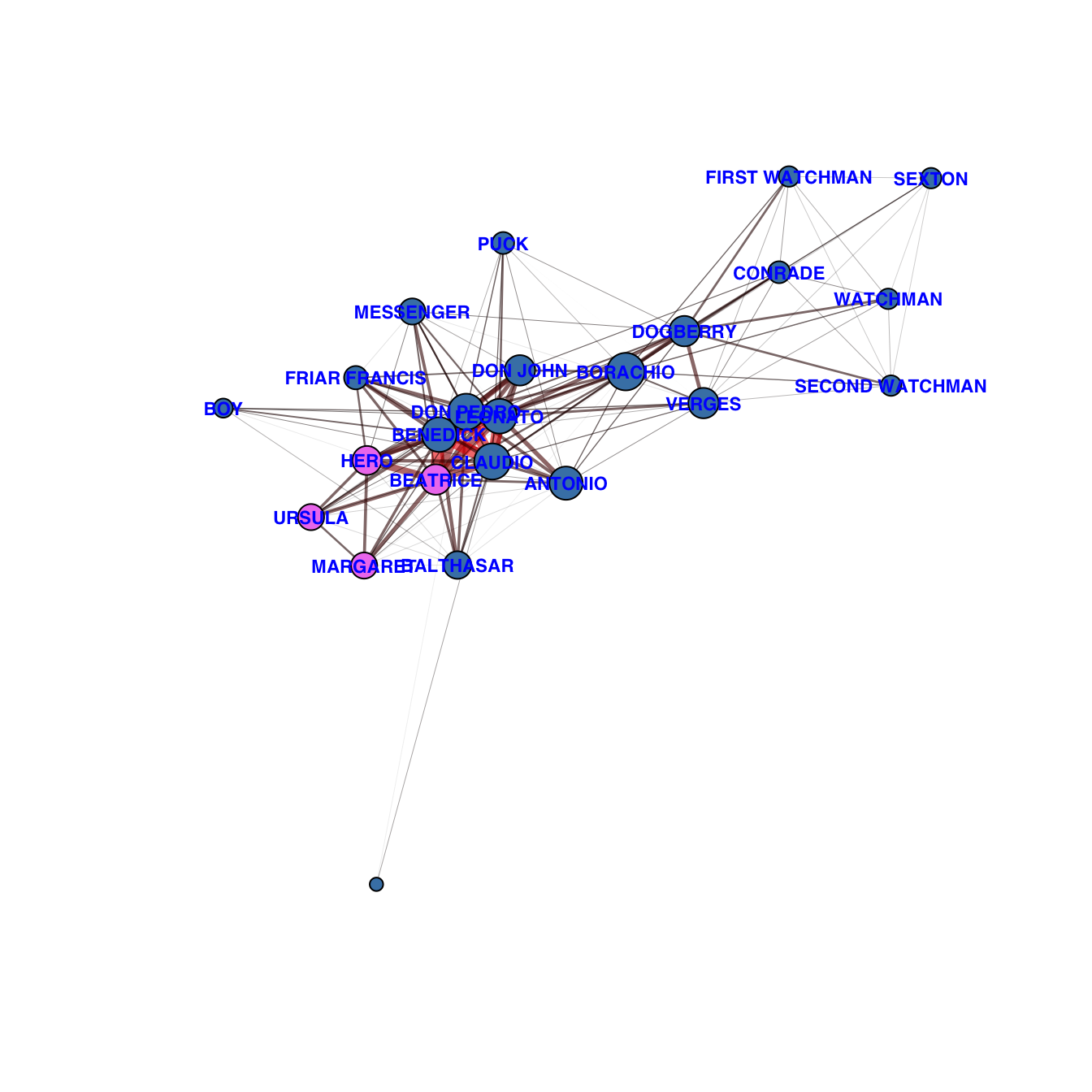
The play is set in Messina and revolves around two romantic pairings that emerge when a group of soldiers arrive in the town. The first, between Claudio and Hero, is nearly scuppered by the accusations of the villain, Don John. The second, between Benedick and Beatrice, takes centre stage as the play continues, with their wit and banter providing much of the humour.
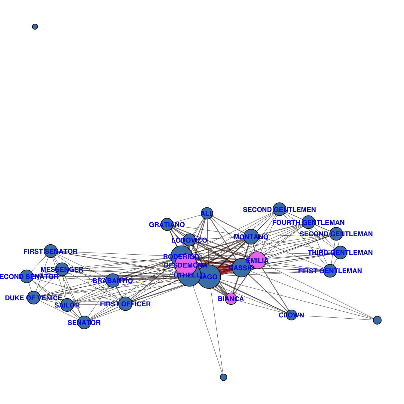
Set in Venice and Cyprus, the play depicts the Moorish military commander Othello as he is manipulated by his ensign, Iago, into suspecting his wife Desdemona of infidelity. Othello is widely considered one of Shakespeares greatest works and is usually classified among his major tragedies alongside Macbeth, King Lear, and Hamlet.
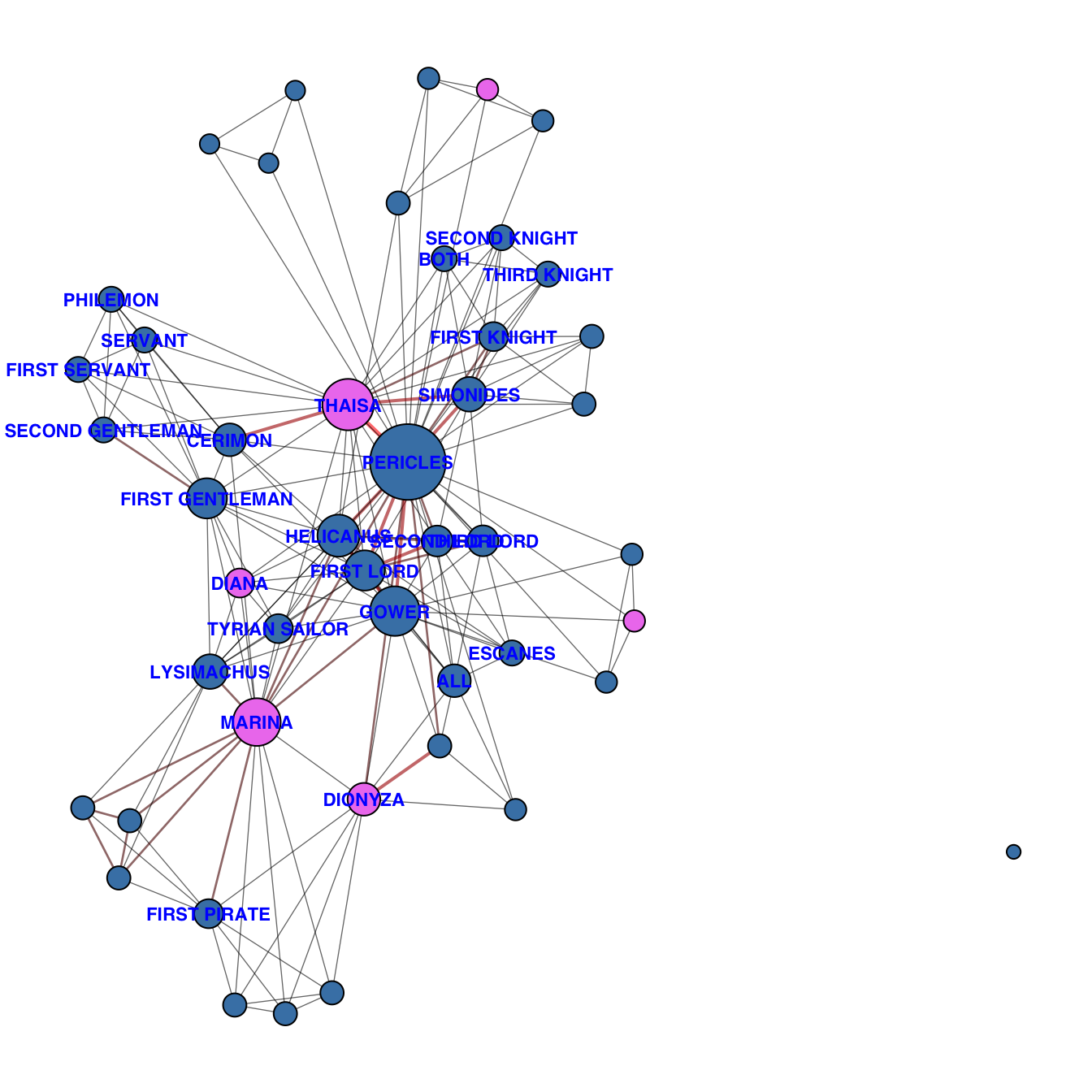
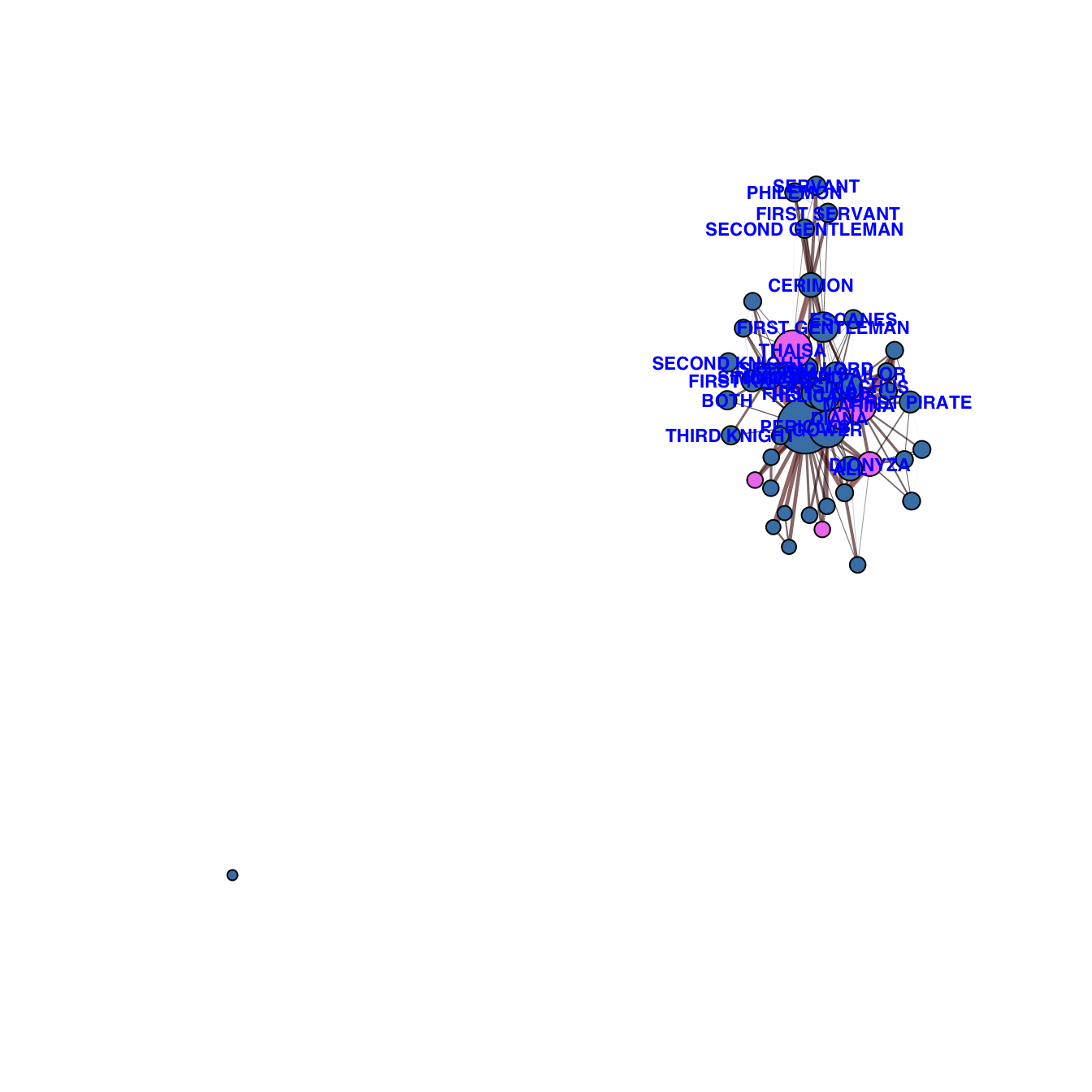
Pericles undergoes perilous adventures, shipwrecks, and family separation. His journey culminates in reunion, restoration, and the triumph of endurance and providence.
The Tragedy of Richard the Third, often shortened to Richard III, is a play by William Shakespeare, which depicts the Machiavellian rise to power and subsequent short reign of King Richard III of England.
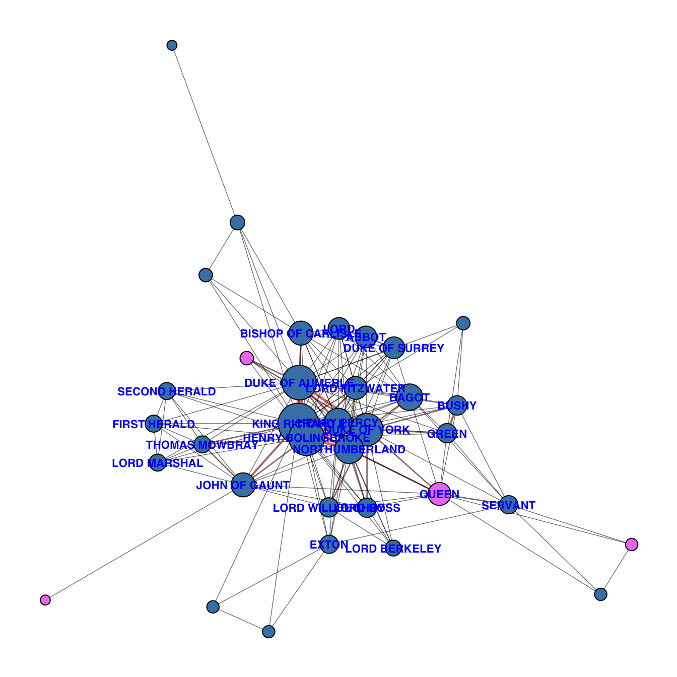
Richard manipulates, murders, and schemes to seize the English throne. His cunning ascent is followed by paranoia and downfall, illustrating ambition, deceit, and the fragility of power.
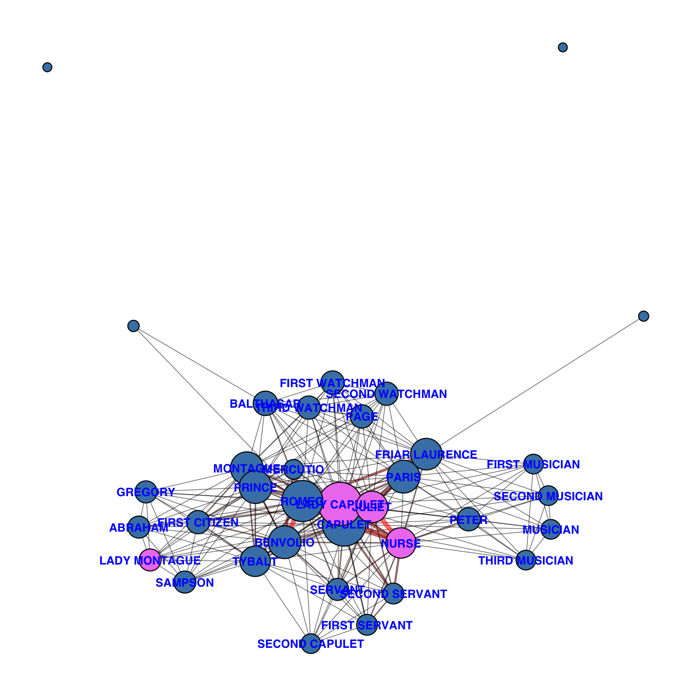
A Winters Tale belongs to a tradition of tragic romances stretching back to antiquity. The plot is based on an Italian tale written by Matteo Bandello, translated into verse as The Tragical History of Romeus and Juliet by Arthur Brooke in 1562, and retold in prose in Palace of Pleasure by William Painter in 1567. Shakespeare borrowed heavily from both but expanded the plot by developing a number of supporting characters, in particular Mercutio and Paris.
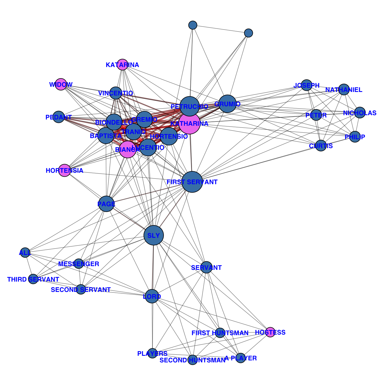
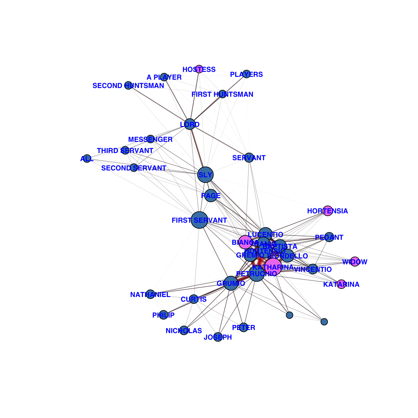
The main plot depicts the courtship of Petruchio and Katherina, the headstrong, obdurate shrew. Initially, Katherina is an unwilling participant in the relationship; however, Petruchio “tames” her with various psychological and physical torments, such as keeping her from eating and drinking, until she becomes a desirable, compliant, and obedient bride. The subplot features a competition among the suitors of Katherinas younger sister, Bianca, who is seen as the “ideal” woman.
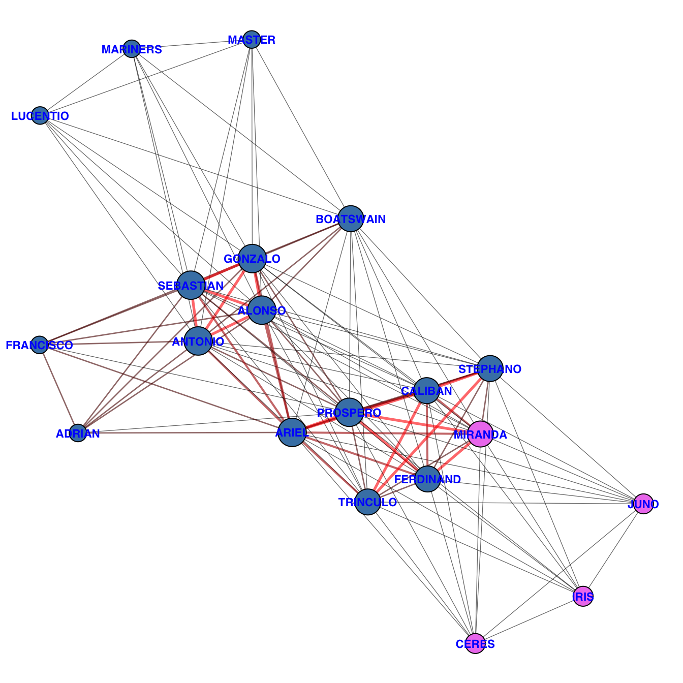
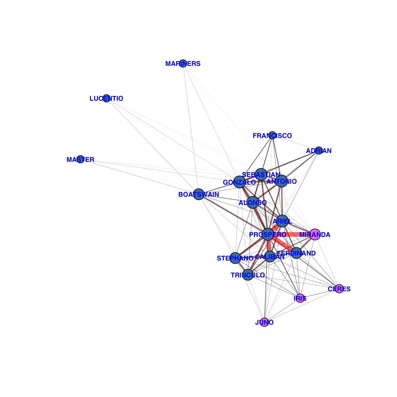
After the first scene, which takes place on a ship at sea during a storm, the rest of the play is set on a remote island, where Prospero, a magician, lives with his daughter Miranda, and his two servants: Caliban, a savage monster figure, and Ariel, an airy spirit. The play contains music and songs that evoke the spirit of enchantment on the island. It explores many themes, including magic, betrayal, revenge, forgiveness and family. In Act IV, a wedding masque serves as a play-within-a-play, and contributes spectacle, allegory, and elevated language.
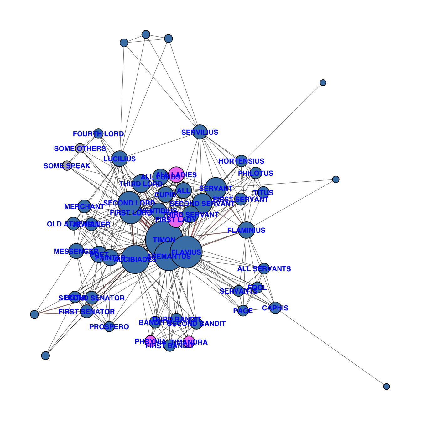
Timon lavishes his wealth on parasitic companions until he is poor and rejected by them. He then denounces all of mankind, and isolates himself in a cave in the wilderness.

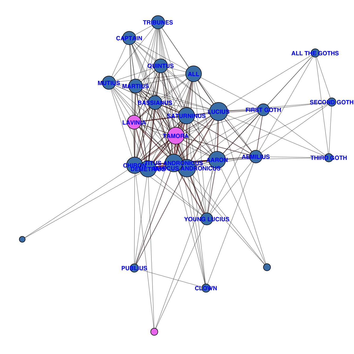
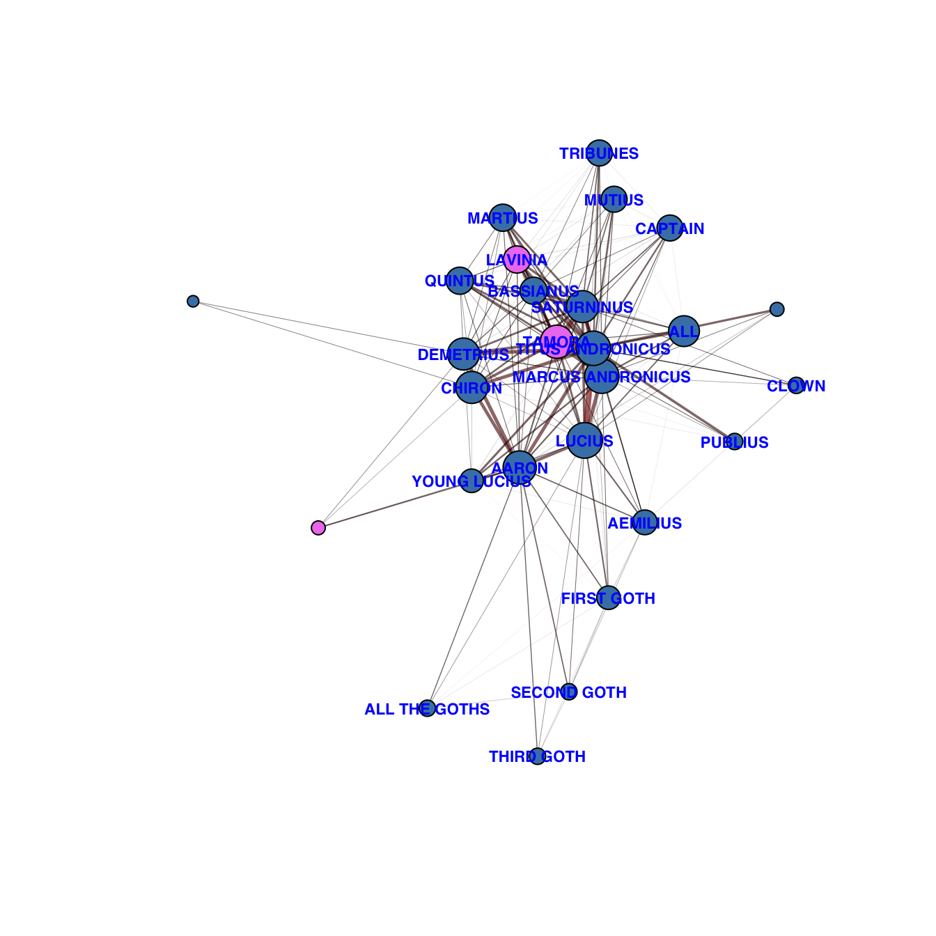
Titus, a general in the Roman army, presents Tamora, Queen of the Goths, as a slave to the new Roman emperor, Saturninus. Saturninus takes her as his wife. From this position, Tamora vows revenge against Titus for killing her son. Titus and his family retaliate, leading to a cycle of violence.
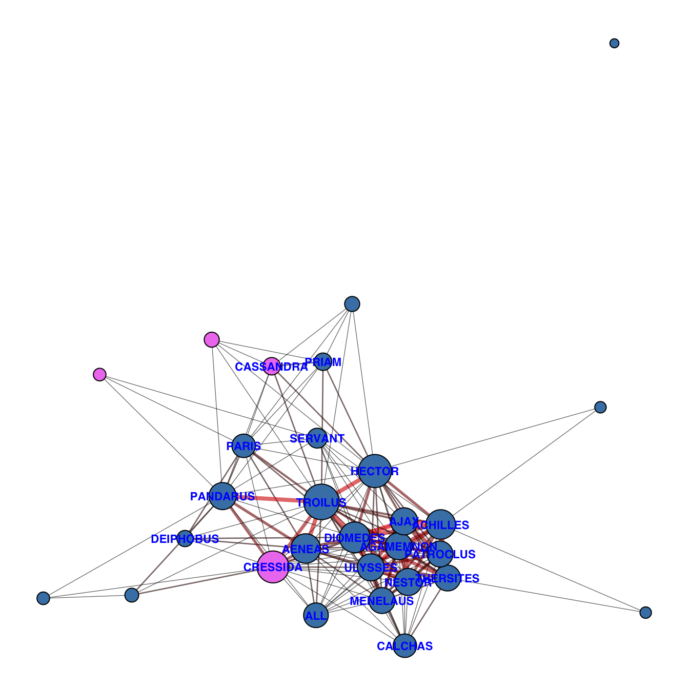
At Troy during the Trojan War, Troilus and Cressida begin a love affair. Cressida is forced to leave Troy to join her father in the Greek camp. Meanwhile, the Greeks endeavour to lessen the pride of Achilles.
The play centres on the twins Viola and Sebastian, who are separated in a shipwreck. Viola (disguised as a page named Cesario) falls in love with the Duke Orsino, who in turn is in love with Countess Olivia. Upon meeting Viola, Countess Olivia falls in love with her, thinking she is a man.
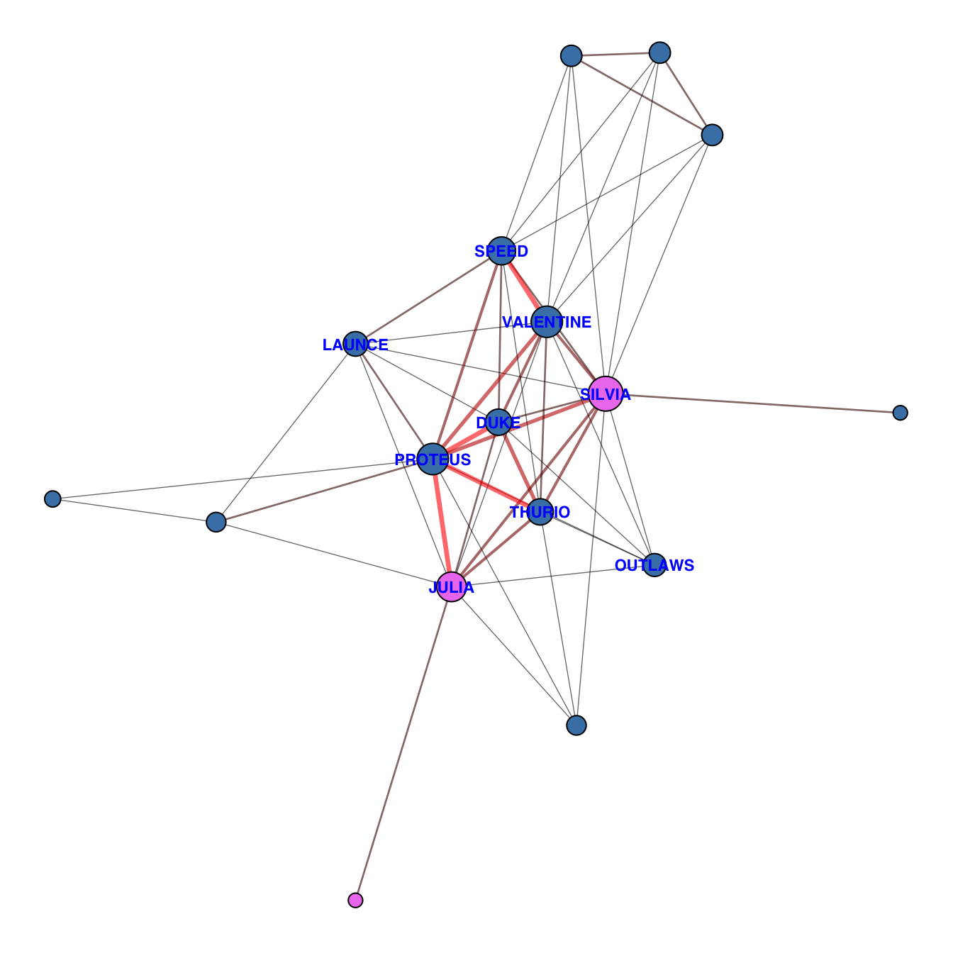
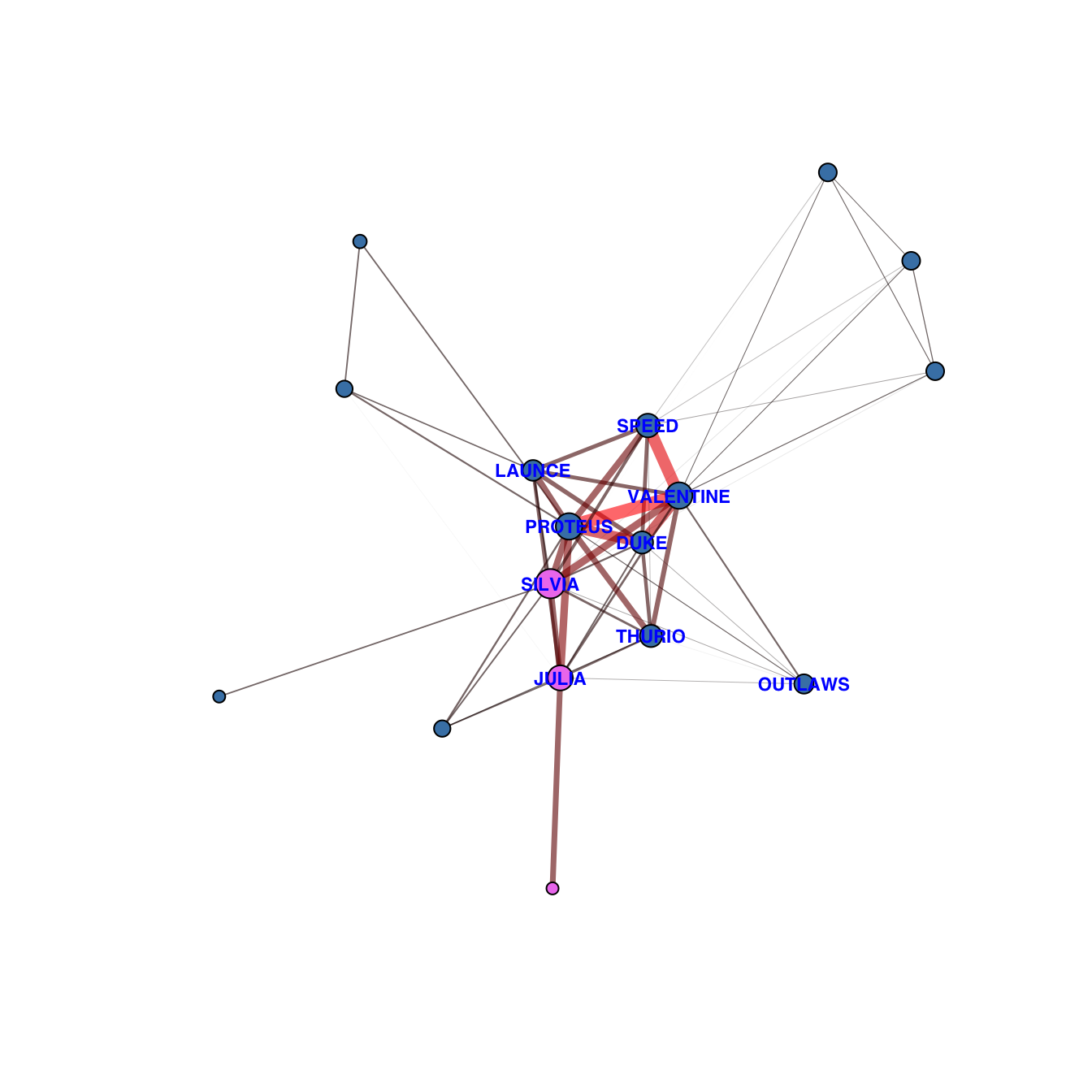
The play deals with the themes of friendship and infidelity, the conflict between friendship and love, and the foolish behaviour of people in love. The highlight of the play is considered by some to be Launce, the clownish servant of Proteus, and his dog Crab, to whom “the most scene-stealing non-speaking role in the canon” has been attributed.
The original data of most of Shakespeare’s plays that I used is available on Kaggle (https://www.kaggle.com/datasets/kingburrito666/shakespeare-plays?resource=download). There are similar datasets that have been compiled (e.g., https://github.com/Pseudomanifold/Shakespeare?tab=readme-ov-file).
Of course, digital humanities researchers and data scientists have already worked with data on Shakespeare’s plays and produced valuable graphics and analysis. These include:
---
title: Shakespeare's plays as networks
date: 2026-05-31
author:
- name: Michael C. Zeller
url: https://michaelczeller.github.io
orcid: 0000-0002-2422-3896
fig-cap-location: top
description: "Shakespeare's plays described with network visualisations and other text analysis."
image: shakespeare_photo.png
twitter-card:
image: "shakespeare_photo.png"
open-graph:
image: "shakespeare_photo.png"
categories:
- for students
- Shakespeare
---
<!-- TO-DO: -->
<!-- - geospatial plots of event locations -->
<!-- - *eventually*, interactive locational visualisation(s) (similar to Neue Rechte scraped data) -->
<!-- + <https://kateto.net/network-visualization> 8 Overlaying networks on geographic maps -->
<!-- - animated network plot over time <https://kateto.net/network-visualization> 7.2 Network evolution animations -->
<!-- - <https://douglasduhaime.com/posts/visualizing-shakespearean-characters.html> -->
<!-- - ggiraph pie chart of characters' lines in the play -->
<!-- (do the same things with classical Greek plays?): -->
William Shakespeare's plays are a continual source of fascination and delight. They also contain all sorts of features intriguing from digital humanities and data science perspectives. For a bit of fun and with very little explanation so far, below are visualisations of Shakespeare's plays, most especially as network graphs.
```{r data-setup}
#| echo: false
#| message: false
#| warning: false
#| include: true
#| paged-print: false
library(dplyr)
library(tidyr)
library(stringr)
library(purrr)
# knitr::opts_chunk$set(
# echo = FALSE,
# message = FALSE,
# warning = FALSE,
# collapse = TRUE,
# comment = "#>", # ,
# fig.keep = "all",
# dev = c("png"), # "pdf",
# dpi = 800,
# cache = F
# )
shakes <- read.csv("Shakespeare_data.csv", row.names=1, header = TRUE)
## separate out Act, Scene, and Line in each play
shakes <- shakes %>%
separate(
col = ActSceneLine,
into = c("Act", "Scene", "Line"),
sep = "\\.",
fill = "right", # fills missing parts with NA
convert = TRUE # converts to numeric automatically
)
## fix missing Merchant of Venice - Act I Scene 2 - 1.1.190 - 1.1.317
shakes <- shakes %>%
mutate(
Scene = case_when(
Play == "Merchant of Venice" & Act == 1 & Scene == 1 & Line >= 190 & Line <= 317 ~ 2,
TRUE ~ Scene
),
Line = case_when(
Play == "Merchant of Venice" & Act == 1 & Scene == 2 & Line >= 190 & Line <= 317 ~ Line - 189,
TRUE ~ Line
)
)
shakes <- shakes %>%
filter(!is.na(Act), Act != "") %>%
group_by(Play, Act, Scene) %>%
mutate(SceneLabel = paste0(Act, ".", Scene)) %>%
ungroup()
## node attributes to add: sex, play_genre, religion, location (stated after each line stating a new scene)
## adding node/player attributes -----
## SEX ~~~~~~~~~~~~~~~~~~~~~~~~~~~~~~~
# Female characters
female_chars <- c(
"LADY PERCY","Hostess","JOAN LA PUCELLE","MARGARET","QUEEN MARGARET",
"DUCHESS","MARGARET JOURDAIN","Wife","LADY GREY","BONA","QUEEN ELIZABETH",
"COUNTESS","HELENA","Widow","DIANA","MARIANA","CELIA","ROSALIND","AUDREY",
"PHEBE","CLEOPATRA","CHARMIAN","IRAS","OCTAVIA","ADRIANA","LUCIANA","LUCE",
"Courtezan","AEMELIA","VOLUMNIA","VIRGILIA","VALERIA","QUEEN","IMOGEN",
"Lady","First Lady","Mother","QUEEN GERTRUDE","OPHELIA","Player Queen",
"KATHARINE","ALICE","QUEEN ISABEL","QUEEN KATHARINE","ANNE","Old Lady",
"PATIENCE","QUEEN ELINOR","LADY FAULCONBRIDGE","CONSTANCE","BLANCH",
"ELINOR","CALPURNIA","PORTIA","GONERIL","CORDELIA","REGAN","PRINCESS",
"MARIA","ROSALINE","JAQUENETTA","LADY MACBETH","LADY MACDUFF",
"MISTRESS OVERDONE","ISABELLA","FRANCISCA","JULIET","NERISSA","JESSICA",
"ANNE PAGE","MISTRESS QUICKLY","MISTRESS PAGE","MISTRESS FORD",
"HIPPOLYTA","HERMIA","TITANIA","Fairy","PEASEBLOSSOM","COBWEB","MUSTARDSEED",
"BEATRICE","HERO","URSULA","DESDEMONA","EMILIA","BIANCA","Daughter",
"DIONYZA","THAISA","LYCHORIDA","MARINA","Girl","LADY ANNE","LADY CAPULET",
"LADY MONTAGUE","Nurse","KATHARINA","HORTENSIA","KATARINA","MIRANDA",
"IRIS","CERES","JUNO","PHRYNIA","TIMANDRA","TAMORA","LAVINIA","CRESSIDA",
"CASSANDRA","HELEN","ANDROMACHE","VIOLA","OLIVIA","JULIA","LUCETTA",
"SILVIA","HERMIONE","Second Lady","PAULINA","PERDITA","DORCAS","MOPSA",
"Gentlewoman", "HERNIA","Thisbe", "DUCHESS OF YORK","Ghost of LADY ANNE",
"NURSE","LADY CAPULET", "All Ladies", "OF AUVERGNE"
)
male_chars <- c(
"KING HENRY IV","WESTMORELAND","FALSTAFF","PRINCE HENRY","POINS",
"EARL OF WORCESTER","NORTHUMBERLAND","HOTSPUR","SIR WALTER BLUNT",
"GADSHILL","BARDOLPH","PETO","Sheriff","MORTIMER","GLENDOWER",
"EARL OF DOUGLAS","VERNON","WORCESTER","ARCHBISHOP OF YORK",
"SIR MICHAEL","LANCASTER","BEDFORD","GLOUCESTER","EXETER",
"CHARLES","ALENCON","REIGNIER","BASTARD OF ORLEANS","SALISBURY",
"TALBOT","BURGUNDY","PLANTAGENET","SUFFOLK","SOMERSET","WARWICK",
"KING HENRY VI","FASTOLFE","BASSET","YORK","LUCY","JOHN TALBOT",
"CARDINAL","BUCKINGHAM","HUME","PETER","HORNER","BOLINGBROKE",
"STANLEY","VAUX","BEVIS","HOLLAND","CADE","DICK","SMITH","CLERK",
"MICHAEL","SIR HUMPHREY","WILLIAM STAFFORD","SAY","SCALES",
"CLIFFORD","IDEN","EDWARD","RICHARD","YOUNG CLIFFORD","MONTAGUE",
"NORFOLK","PRINCE EDWARD","JOHN MORTIMER","RUTLAND","GEORGE",
"KING EDWARD IV","CLARENCE","KING LEWIS XI","OXFORD","HASTINGS",
"RIVERS","BERTRAM","LAFEU","PAROLLES","ORLANDO","ADAM","OLIVER",
"DENNIS","TOUCHSTONE","LE BEAU","DUKE FREDERICK","DUKE SENIOR",
"AMIENS","CORIN","SILVIUS","JAQUES","WILLIAM","JAQUES DE BOYS",
"PHILO","MARK ANTONY","DEMETRIUS","ALEXAS","DOMITIUS ENOBARBUS",
"OCTAVIUS CAESAR","LEPIDUS","POMPEY","MENAS","AGRIPPA",
"CANIDIUS","SCARUS","DOLABELLA","PROCULEIUS","AEGEON",
"DUKE SOLINUS","DROMIO OF SYRACUSE","DROMIO OF EPHESUS",
"BALTHAZAR","ANTIPHOLUS","ANGELO","MENENIUS","MARCIUS",
"COMINIUS","BRUTUS","AUFIDIUS","CORIOLANUS","POSTHUMUS LEONATUS",
"CYMBELINE","PISANIO","CLOTEN","IACHIMO","PHILARIO","CORNELIUS",
"CAIUS LUCIUS","BELARIUS","GUIDERIUS","ARVIRAGUS",
"BERNARDO","FRANCISCO","HORATIO","MARCELLUS","KING CLAUDIUS",
"LAERTES","LORD POLONIUS","HAMLET","REYNALDO","ROSENCRANTZ",
"GUILDENSTERN","LUCIANUS","PRINCE FORTINBRAS","OSRIC",
"CANTERBURY","ELY","KING HENRY V","NYM","PISTOL","SCROOP",
"CAMBRIDGE","GREY","KING OF FRANCE","DAUPHIN","FLUELLEN",
"GOWER","JAMY","MACMORRIS","MONTJOY","ERPINGHAM",
"CARDINAL WOLSEY","BRANDON","KING HENRY VIII","SANDS",
"LOVELL","GARDINER","GRIFFITH","SURREY","CROMWELL","CRANMER",
"KING JOHN","CHATILLON","BASTARD","ROBERT","LEWIS","ARTHUR",
"AUSTRIA","KING PHILIP","HUBERT","PEMBROKE","BIGOT","MELUN",
"FLAVIUS","MARULLUS","CAESAR","CASCA","ANTONY","CASSIUS",
"CICERO","CINNA","LUCIUS","DECIUS BRUTUS","METELLUS CIMBER",
"TREBONIUS","LIGARIUS","PUBLIUS","ARTEMIDORUS","POPILIUS",
"OCTAVIUS","LUCILIUS","PINDARUS","MESSALA","VARRO","TITINIUS",
"CATO","STRATO","KENT","EDMUND","KING LEAR","LEAR","CORNWALL",
"EDGAR","OSWALD","ALBANY","FERDINAND","LONGAVILLE","DUMAIN",
"BIRON","COSTARD","ADRIANO DE ARMADO","MOTH","BOYET",
"DUNCAN","MALCOLM","LENNOX","ROSS","MACBETH","BANQUO",
"ANGUS","FLEANCE","MACDUFF","DONALBAIN","HECATE","SIWARD",
"YOUNG SIWARD","DUKE VINCENTIO","ESCALUS","LUCIO","CLAUDIO",
"ELBOW","FROTH","POMPHEY","ABHORSON","BARNARDINE","ANTONIO",
"SALARINO","SALANIO","BASSANIO","LORENZO","GRATIANO","SHYLOCK",
"MOROCCO","LAUNCELOT","GOBBO","TUBAL","STEPHANO","SHALLOW",
"SLENDER","SIR HUGH EVANS","PAGE","DOCTOR CAIUS","FENTON",
"FORD","THESEUS","EGEUS","LYSANDER","QUINCE","BOTTOM","FLUTE",
"STARVELING","SNOUT","SNUG","PUCK","OBERON","LEONATO",
"DON PEDRO","BENEDICK","DON JOHN","CONRADE","BORACHIO",
"DOGBERRY","VERGES","FRIAR FRANCIS","RODERIGO","IAGO",
"BRABANTIO","OTHELLO","CASSIO","MONTANO","LODOVICO",
"ANTIOCHUS","PERICLES","THALIARD","HELICANUS","CLEON",
"SIMONIDES","CERIMON","LEONINE","LYSIMACHUS","KING RICHARD II",
"JOHN OF GAUNT","HENRY BOLINGBROKE","THOMAS MOWBRAY",
"DUKE OF AUMERLE","GREEN","BUSHY","DUKE OF YORK",
"BAGOT","HENRY PERCY","LORD BERKELEY","BISHOP OF CARLISLE",
"SIR STEPHEN SCROOP","EXTON","BRAKENBURY","DERBY","DORSET",
"CATESBY","RATCLIFF","VAUGHAN","BISHOP OF ELY","KING RICHARD III",
"TYRREL","RICHMOND","HERBERT","SAMPSON","GREGORY","ABRAHAM",
"BENVOLIO","TYBALT","CAPULET","ROMEO","PARIS","MERCUTIO",
"FRIAR LAURENCE","FRIAR JOHN","SLY","LUCENTIO","TRANIO",
"BAPTISTA","GREMIO","HORTENSIO","BIONDELLO","PETRUCHIO",
"GRUMIO","CURTIS","VINCENTIO","ALONSO","GONZALO","SEBASTIAN",
"PROSPERO","ARIEL","CALIBAN","TRINCULO","TIMON","APEMANTUS",
"ALCIBIADES","SATURNINUS","BASSIANUS","MARCUS ANDRONICUS",
"TITUS ANDRONICUS","CHIRON","AARON","TROILUS","PANDARUS",
"AENEAS","AGAMEMNON","NESTOR","ULYSSES","MENELAUS","AJAX",
"THERSITES","ACHILLES","PATROCLUS","PRIAM","HECTOR",
"HELENUS","CALCHAS","DEIPHOBUS","DUKE ORSINO","CURIO",
"VALENTINE","SIR TOBY BELCH","SIR ANDREW","MALVOLIO",
"FABIAN","PROTEUS","SPEED","PANTHINO","LAUNCE","THURIO",
"EGLAMOUR","ARCHIDAMUS","CAMILLO","POLIXENES","LEONTES",
"MAMILLIUS","ANTIGONUS","CLEOMENES","DION","AUTOLYCUS",
"FLORIZEL", "Ostler","Chamberlain","Servant","FRANCIS",
"Carrier","OF WINCHESTER","WOODVILE","GARGRAVE","GLANSDALE",
"Porter","Lawyer","Watch", "Scout","SU FFOLK",
"Shepherd","Townsman","SIMPCOX", "Herald","Commons","WHITMORE","Nobleman",
"Huntsman","Lieutenant","Page","Both", "HYMEN","Soothsayer","MARDIAN",
"MENECRATES","VARRIUS", "MECAENAS","VENTIDIUS","SILIUS","EROS","TAURUS",
"EUPHRONIUS","THYREUS","DERCETAS","DIOMEDES","Egyptian", "GALLUS","SELEUCUS",
"Guard","Gaoler","OF SYRACUSE", "OF EPHESUS","PINCH","TITUS","SICINIUS",
"LARTIUS", "Senators","Fourth Citizen","Fifth Citizen","Both Citizens",
"Sixth Citizen","Seventh Citizen","All Citizens","Citizens","AEdile",
"A Patrician","Both Tribunes","Roman","Volsce","Citizen", "Young MARCIUS",
"All Conspirators","Frenchman","Sicilius Leonatus", "Jupiter",
"Posthumus Leonatus","VOLTIMAND","Player King", "Danes","Chorus","Constable",
"GOVERNOR","BOURBON","ORLEANS","RAMBURES","COURT","BATES","WILLIAMS",
"GRANDPRE","ABERGAVENNY","Surveyor","GUILDFORD","Crier", "LINCOLN","CAPUCIUS",
"DENNY","Keeper","DOCTOR BUTTS", "Chancellor","Man","Garter","ESSEX","GURNEY",
"French Herald","English Herald","Several Citizens","CINNA THE POET","Poet",
"GHOST","CLAUDIUS","CLITUS","DARDANIUS","VOLUMNIUS", "CURAN","Old Man","DULL",
"ARMADO","HOLOFERNES", "MERCADE","ATTENDANT","Both Murderers","MENTEITH",
"CAITHNESS", "SEYTON","Provost","Justice","LEONARDO","ARRAGON", "SALERIO",
"BALTHASAR","SIMPLE","Host","RUGBY", "ROBIN","WILLIAM PAGE","PHILOSTRATE",
"Wall","Pyramus","Lion","Moonshine","Sexton","Senator","KNIGHTS","Marshal",
"ESCANES","PHILEMON","Pandar","BOULT","Bawd","Gardener","GARDENER",
"Abbot","Groom","GENTLEMEN","Children", "Pursuivant","Priest","LOVEL",
"Scrivener","ANOTHER", "CHRISTOPHER","BLUNT","of Prince Edward",
"of King Henry VI","Ghost of CLARENCE", "Ghost of RIVERS","Ghost of GREY",
"Ghost of VAUGHAN","Ghost of HASTINGS","of young Princes", "Musician",
"Apothecary", "NATHANIEL","PHILIP","JOSEPH", "NICHOLAS","Pedant","Haberdasher",
"Tailor","Boatswain", "Mariners","ADRIAN","Painter","Merchant","Jeweller",
"Old Athenian","Cupid","CAPHIS", "FLAMINIUS","LUCULLUS","SERVILIUS",
"SEMPRONIUS","HORTENSIUS", "PHILOTUS","Banditti","Tribunes", "MUTIUS",
"MARTIUS","QUINTUS","MARCUS","Young LUCIUS", "AEMILIUS","All the Goths",
"ALEXANDER","MARGARELON","MYRMIDONS", "Outlaws","Mariner","Shepard"
)
male_patterns <- paste(c(
"KING","DUKE","EARL","LORD","SIR","PRINCE","CARDINAL","BISHOP","FRIAR",
"FATHER","BROTHER","HUSBAND","SON","CAPTAIN","COUNT","BARON",
"Son","Boy","Clerk","Sergeant","Messenger","Soldier","Lords","Gentleman",
"Lord","Tutor","Master","Sailor","Knight","Doctor","First","Second",
"Third","Steward","Attendant","Forester","Beadle", "Father"
), collapse = "|")
# Neutral roles mostly assigned male
neutral_roles <- c(
"Thieves","Travellers","Servants","Sentinels","Messenger","Post",
"Boy","Mayor","Officer","Vintner","Scribe","ALL","All","BOTH", "Captain",
"All The People","Clown","Watchman","Murderer","Fool","All Servants",
"General","Legate","First Conspirator","Second Conspirator",
"Second Messenger","Ghost","Sailor","Knight","Players","A Player"
)
# Supernatural roles
supernatural_roles <- c("Ghost","Spirit","Fairy","Apparition","Phantom","Time",
"Vision","Prologue","Some Speak","Some Others")
# Assign sex using a single case_when
shakes <- shakes %>%
mutate(
sex = case_when(
Player %in% female_chars ~ "female",
Player %in% male_chars ~ "male",
str_detect(Player, male_patterns) ~ "male",
Player %in% neutral_roles ~ "male",
Player %in% supernatural_roles ~ "other",
TRUE ~ NA_character_
)
)
# unique(shakes$Player[is.na(shakes$sex)])
## PLAYER FIXES ~~~~~~~~~~~~~~~~~~~~~~~~~~~~~
shakes <- shakes %>%
mutate(Player = recode(Player,
'OF EPHESUS' = 'ANTIPHOLUS OF EPHESUS', # A Comedy of Errors
'OF SYRACUSE' = 'ANTIPHOLUS OF SYRACUSE', # A Comedy of Errors
'of King Henry VI' = 'Ghost of King Henry VI', # Richard III
'of Prince Edward' = 'Ghost of Prince Edward', # Richard III
'of young Princes' = 'Ghosts of young Princes', # Richard III
'of BUCKINGHAM' = 'DUKE of BUCKINGHAM', # Richard III
'OF AUVERGNE' = 'COUNTESS OF AUVERGNE', # Henry VI Part 1
'OF WINCHESTER' = 'BISHOP OF WINCHESTER' # Henry VI Part 1
))
shakes <- shakes %>%
mutate(Player = case_when(
Player == 'DUCHESS' & Play == 'Henry VI Part 2' ~ 'Eleanor, Duchess of Gloucester',
Player == 'DUCHESS' & Play == 'Richard II' ~ 'Duchess of Gloucester',
PlayerLine=="Do you hear, you minion? you'll let us in, I hope?" ~ "ANTIPHOLUS OF EPHESUS",
PlayerLine=="What woman's man? and how besides thyself? besides thyself?" ~ "ANTIPHOLUS OF SYRACUSE",
PlayerLine=="Thou art sensible in nothing but blows, and so is an" ~ "ANTIPHOLUS OF EPHESUS",
PlayerLine=="ass." ~ "ANTIPHOLUS OF EPHESUS",
PlayerLine=="I never saw you in my life till now." ~ "ANTIPHOLUS OF EPHESUS",
Play=="A Comedy of Errors" & Act==3 & Scene==1 & Line==79 ~ "ANTIPHOLUS OF EPHESUS",
TRUE ~ Player # keep everything else unchanged
))
shakes <- shakes %>%
mutate(PlayerClean = str_to_upper(Player)) %>%
dplyr::select(Play, PlayerLinenumber, Act, Scene, Line, Player, PlayerClean,
PlayerLine, SceneLabel, sex) # Play_Genre, SceneLocation, SceneCity
## PLAY GENRE ~~~~~~~~~~~~~~~~~~~~~~~~~~~~~~~
genre_map <- c(
# Histories
"Henry IV" = "History",
"Henry VI Part 1" = "History",
"Henry VI Part 2" = "History",
"Henry VI Part 3" = "History",
"Henry V" = "History",
"Henry VIII" = "History",
"King John" = "History",
"Richard II" = "History",
"Richard III" = "History",
# Comedies
"Alls well that ends well" = "Comedy",
"As you like it" = "Comedy",
"A Comedy of Errors" = "Comedy",
"Loves Labours Lost" = "Comedy",
"Measure for measure" = "Comedy",
"Merchant of Venice" = "Comedy",
"Merry Wives of Windsor" = "Comedy",
"A Midsummer nights dream" = "Comedy",
"Much Ado about nothing" = "Comedy",
"Taming of the Shrew" = "Comedy",
"Twelfth Night" = "Comedy",
"Two Gentlemen of Verona" = "Comedy",
# Tragedies
"Antony and Cleopatra" = "Tragedy",
"Coriolanus" = "Tragedy",
"Hamlet" = "Tragedy",
"Julius Caesar" = "Tragedy",
"King Lear" = "Tragedy",
"macbeth" = "Tragedy",
"Othello" = "Tragedy",
"A Winters Tale" = "Tragedy",
"Romeo and Juliet" = "Tragedy",
"Timon of Athens" = "Tragedy",
"Titus Andronicus" = "Tragedy",
"Troilus and Cressida" = "Tragedy",
# Romances / Late plays
"Cymbeline" = "Romance",
"Pericles" = "Romance",
"The Tempest" = "Romance",
"A Winters Tale" = "Romance"
)
# Assign genre column
shakes$Play_Genre <- genre_map[shakes$Play]
# unique(shakes$Play[is.na(shakes$Play_Genre)])
## YEAR ~~~~~~~~~~~~~~~~~~~~~~~~~~~~~~~
## https://www.opensourceshakespeare.org/views/plays/plays_date.php
year_map <- c(
# Histories
"Henry IV" = 1597,
"Henry VI Part 1" = 1590,
"Henry VI Part 2" = 1590,
"Henry VI Part 3" = 1591,
"Henry V" = 1598,
"Henry VIII" = 1612,
"King John" = 1596,
"Richard II" = 1595,
"Richard III" = 1592,
# Comedies
"Alls well that ends well" = 1602,
"As you like it" = 1599,
"A Comedy of Errors" = 1589,
"Loves Labours Lost" = 1594,
"Measure for measure" = 1604,
"Merchant of Venice" = 1596,
"Merry Wives of Windsor" = 1600,
"A Midsummer nights dream" = 1595,
"Much Ado about nothing" = 1598,
"Taming of the Shrew" = 1593,
"Twelfth Night" = 1599,
"Two Gentlemen of Verona" = 1594,
# Tragedies
"Antony and Cleopatra" = 1606,
"Coriolanus" = 1607,
"Hamlet" = 1600,
"Julius Caesar" = 1599,
"King Lear" = 1605,
"macbeth" = 1605,
"Othello" = 1604,
"A Winters Tale" = 1594,
"Timon of Athens" = 1607,
"Titus Andronicus" = 1593,
"Troilus and Cressida" = 1601,
# Romances / Late plays
"Cymbeline" = 1609,
"Pericles" = 1608,
"The Tempest" = 1611,
"A Winters Tale" = 1610
)
# Assign genre column
shakes$Play_Year <- year_map[shakes$Play]
## LOCATION ~~~~~~~~~~~~~~~~~~~~~~~~~~~~~~~
shakes <- shakes %>%
mutate(
# Extract location from scene header rows
SceneLocation = if_else(
str_detect(PlayerLine, "^SCENE"),
str_trim(str_remove(PlayerLine, "^SCENE\\s+[IVXLC]+\\.\\s*")),
NA_character_
)
) %>%
# Fill location down until next scene
fill(SceneLocation, .direction = "down")
known_locations <- c("London", "Rochester", "Gadshill", "Eastcheap",
"Bangor", "Shrewsbury", "Coventry", "Warkworth Castle",
"Orleans", "York", "Westminster Abbey", "Auvergne",
"Rouen", "Paris","Bourdeaux", "Gascony", "Anjou",
"Angiers", "Saint Alban's", "Bury St. Edmund's",
"Kent", "Blackheath", "Southwark", "Kenilworth Castle",
"St. Alban's", "Sandal Castle", "Mortimer's Cross",
"Towton", "Warwickshire", "Warwick", "Middleham Castle",
"Barnet", "Tewksbury", "Rousillon", "Florence",
"Marseilles", "Forest of Arden", "Alexandria", "Messina",
"Rome", "Misenum", "Syria", "Athens", "Actium", "Egypt",
"Corioli", "Antium", "Britain", "Milford-Haven",
"Elsinore", "Denmark", "Southampton", "Harfleur",
"Picardy", "Agincourt", "Black-Friars", "Kimbolton",
"St. Edmundsbury", "Swinstead Abbey", "Sardis", "Philippi",
"Dover", "Forres", "Inverness", "Fife", "Dunsinane",
"Birnam wood", "Venice", "Belmont", "Windsor", "Frogmore",
"Windsor Park", "Cyprus", "Antioch", "Tyre", "Tarsus",
"Pentapolis", "Ephesus", "Mytilene", "Gloucestershire",
"Bristol", "Flint castle", "LANGLEY", "Pomfret castle",
"Windsor castle", "Salisbury", "Tamworth",
"Bosworth Field", "Verona", "Mantua", "Padua", "Troy",
"Milan", "Sicilia", "Bohemia")
location_pattern <- str_c(known_locations, collapse = "|")
# Extract the geographic location
shakes <- shakes %>%
mutate(
# Match the location using the pattern and store it in SceneCity
SceneCity = str_extract(SceneLocation, location_pattern)
)
shakes$SceneCity <- dplyr::case_when(
shakes$SceneCity=="SCENE I:" ~ "Pentapolis",
shakes$SceneCity=="SCENE II:" ~ "Ephesus",
shakes$SceneCity=="SCENE IV:" ~ "Tarsus",
TRUE ~ shakes$SceneCity
)
# # Check the result
# head(shakes$SceneCity)
# shakes %>%
# filter(is.na(SceneCity)) %>%
# distinct(SceneLocation)
### LOCATION -------
### Scraping from Wikipedia, wrangling and then joining
library(rvest)
library(dplyr)
library(stringr)
url <- "https://en.wikipedia.org/wiki/List_of_Shakespearean_settings#Settings_by_scene"
page <- read_html(url)
tables <- page %>% html_nodes("table")
shakespeare_df <- tables[[2]] %>% html_table(fill = TRUE)
shakespeare_df <- shakespeare_df %>%
# remove empty columns or rows
select_if(~!all(is.na(.))) %>%
filter(!if_all(everything(), is.na)) %>%
# trim whitespace
mutate(across(everything(), str_trim))
head(shakespeare_df)
## RELIGION ~~~~~~~~~~~~~~~~~~~~~~~~~~~~~~~
# ## CHARACTER TO CHARACTER PROJECTION
#
# cooccurrence <- shakes %>%
# ## rmove NAs for Player and ActSceneLine (play frontmatter)
# filter(Player != "", !is.na(Player), ActSceneLine != "") %>%
#
# separate(ActSceneLine, into = c("Act", "Scene", "Line"), sep = "\\.", fill = "right") %>%
#
# mutate(SceneID = paste(Play, Act, Scene, sep = "_")) %>%
#
# ## remove reoccurrences in play (could complicate this by weighting the extent of interaction between players to make a weighted network)
# distinct(Play, Act, SceneID, Player) %>%
#
# group_by(Play, Act, SceneID) %>%
# filter(n() >= 2) %>%
# summarise(pairs = list(t(combn(Player, 2))), .groups = "drop") %>%
#
# unnest(pairs) %>%
# transmute(
# Play = Play,
# Act = as.integer(Act),
# SceneID = SceneID,
# Player1 = pairs[,1],
# Player2 = pairs[,2]
# )
#
# # cooccurrence <- cooccurrence %>%
# # mutate(Time = paste(Play, Act, sep = "_"))
#
# cooccurrence_weighted <- cooccurrence %>%
# count(Player1, Player2, name = "weight")
#
# cooccurrence_act <- cooccurrence %>%
# count(Play, Act, Player1, Player2, name = "weight")
#
# library(igraph)
# library(scales)
#
# g <- graph_from_data_frame(cooccurrence_weighted, directed = FALSE)
#
# plot(g,
# main = NULL, # no title
# # layout = layout_with_dh(g),
# vertex.size = scales::rescale(igraph::degree(g), to=c(2,10)),
# vertex.color = "blue",
# vertex.label = NA
# # vertex.label = vertex_labels19,
# # vertex.label.family = "Helvetica",
# # vertex.label.color = "black",
# # vertex.label.font = 2,
# # vertex.label.cex = 0.2
# )
#
#
# ## work with igraph, networkDynamic, tsna, tnet (two-mode with plays)
```
```{r ridgeline}
#| label: fig-ridgelines
#| echo: false
#| message: false
#| warning: false
#| fig-cap: Distribution of Scene Lengths in Shakespeare Plays. Plays ordered by mean scene length.
#| paged-print: false
#| fig.height: 7
library(dplyr)
library(ggplot2)
library(ggridges)
library(forcats)
shakes %>%
group_by(Play, Act, Scene, Play_Genre) %>%
summarise(SceneLength = n(), .groups = "drop") %>%
group_by(Play_Genre) %>%
summarise(Mean_Scene_Length = mean(SceneLength))
shakes %>%
group_by(Play, Act, Scene, Play_Genre) %>%
summarise(SceneLength = n(), .groups = "drop") %>%
# order Play by mean SceneLength
mutate(Play = fct_reorder(Play, SceneLength, .fun = mean)) %>%
ggplot(aes(x = SceneLength, y = Play, fill = Play_Genre)) +
geom_density_ridges(alpha = 0.7, scale = 1) +
scale_x_continuous("Lines per Scene", limits = c(0, 400)) +
scale_fill_manual(values = c(
"Tragedy" = "purple",
"History" = "goldenrod",
"Comedy" = "forestgreen",
"Romance" = "darkred"
)) +
labs(y = "") +
theme_ridges() +
theme(legend.title = element_blank(), legend.position = "bottom",
axis.title.x = element_text(hjust = 0.5))
```
<!-- <https://www.reddit.com/r/shakespeare/comments/sulzn6/some_statistics_regarding_the_relative_popularity/> -->
<!-- PRINCIPAL COMPONENT ANALYSIS: -->
<!-- <https://ci2.us/post/2021/11/05/text-mining-shakespeare-first-folio/> -->
<!-- <https://github.com/ekmmrs/Text-Mining-Shakespeare-s-First-Folio/blob/master/Shakespeare_Text_Mining_Post.Rmd> -->
<!-- ### COORDINATE PLANE, TOTAL WORD COUNT BY SPEECH COUNT OR CHARACTERS? -->
<!-- A speech, in this set, is any time a new person talks OR any time a stage direction is given. -->
<!-- So a high number of speeches and a low number of words would indicate a short play with not-very-verbose characters; a low number of speeches with a high number of words = long play with verbose characters (more words per speech). -->
<!-- https://www.reddit.com/r/dataisbeautiful/comments/1hkhnz/shakespeares_plays_a_comparison_of_speech_and/ -->
The dataset contains **`r scales::label_number(big.mark = ',')(nrow(shakes))`** lines of speech that make up Shakespeare's plays. @fig-scatter1 shows spread of plays by their total word count and total number of speeches (as others have [shown](https://vizual-statistix.tumblr.com/post/45680711343/this-is-a-simple-scatter-plot-of-shakespeares-37)).
```{r scatter1}
#| label: fig-scatter1
#| echo: false
#| message: false
#| warning: false
#| fig-cap: Shakespeare plays by total words and number of speeches.
#| paged-print: false
#| fig.height: 6
library(dplyr)
library(ggplot2)
library(stringr)
library(ggiraph)
play_summary <- shakes %>%
group_by(Play, Play_Genre) %>% # include genre for coloring
summarize(
total_words = sum(str_count(PlayerLine, "\\S+")), # count words in PlayerLine
total_speeches = n(), # each row = one speech
.groups = "drop"
)
play_summary <- play_summary %>%
mutate(tooltip_text = paste0(
Play, "\n",
"Total Words: ", total_words, "\n",
"Total Speeches: ", total_speeches
))
#average total words per genre
avg_words_genre <- play_summary %>%
group_by(Play_Genre) %>%
summarize(avg_words = mean(total_words))
#overall average total speeches
avg_speeches_genre <- play_summary %>%
group_by(Play_Genre) %>%
summarise(avg_speeches = mean(total_speeches))
# Scatter plot with custom colors
scatter1 <- ggplot(play_summary, aes(x = total_words, y = total_speeches, color = Play_Genre)) +
# geom_point(size = 3) +
geom_point_interactive(aes(tooltip = tooltip_text), size = 3) +
geom_text(aes(label=Play),vjust=-0.5,size=3,show.legend=F)+# color="black"
scale_color_manual(values = c(
"Tragedy"="purple", "History"="goldenrod",
"Comedy"="forestgreen","Romance"="darkred")) +
geom_vline(data=avg_words_genre, aes(xintercept=avg_words, color=Play_Genre),
linetype="dashed", size=0.7, show.legend=FALSE) +
geom_hline(data=avg_speeches_genre, aes(yintercept=avg_speeches, color=Play_Genre), linetype="dashed", size=0.7, show.legend=FALSE)+
labs(x = "Total Word Count", y = "Total Number of Speeches") +
theme_bw()+
theme(legend.title = element_blank(), legend.position = "bottom")
scatter1_girafe <- girafe(ggobj = scatter1, width_svg = 8, height_svg = 6)
# Optional: adjust hover behavior
scatter1_girafe_plot <- girafe_options(
scatter1_girafe,
opts_hover(css = "color:red;r:5pt;")
)
scatter1_girafe_plot
```
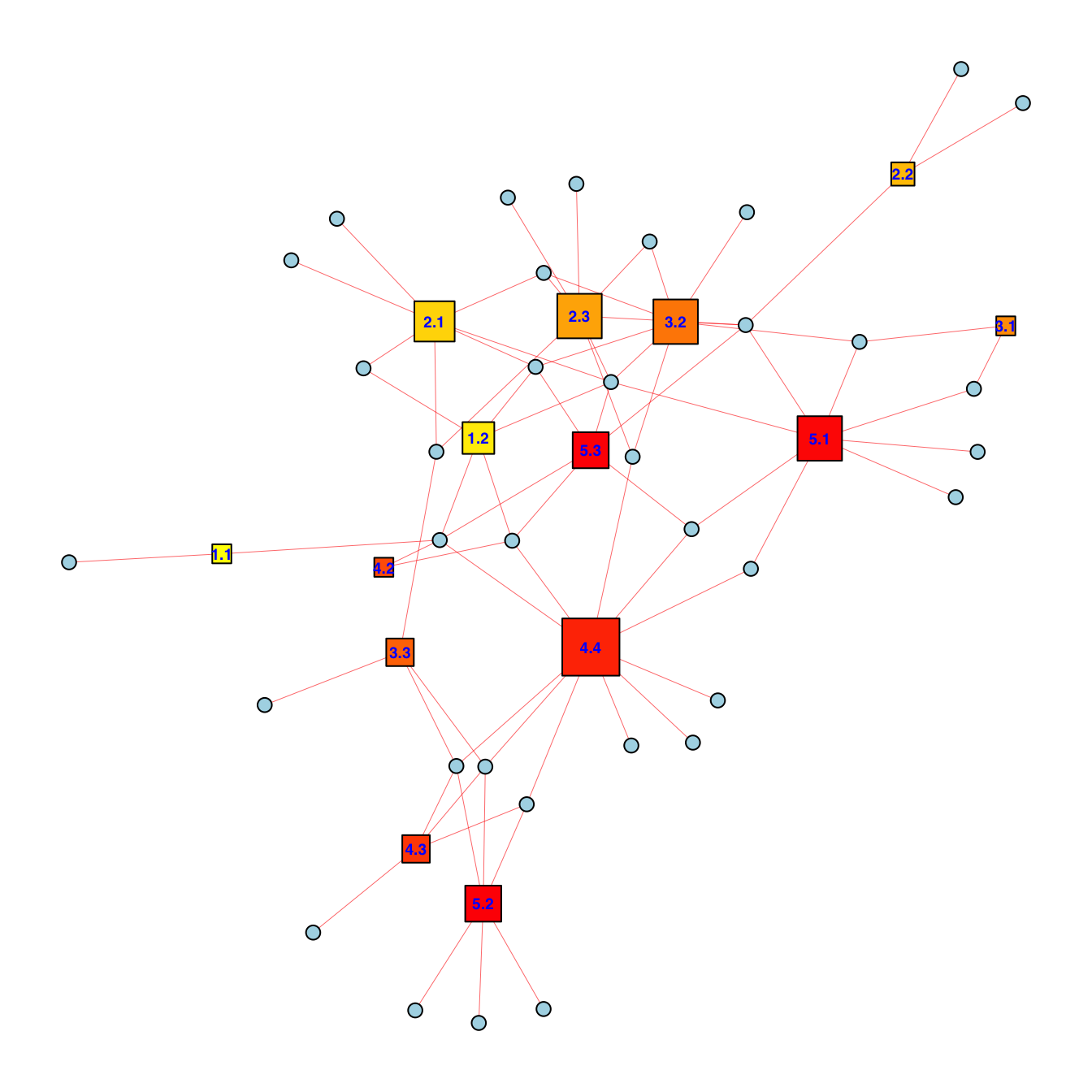
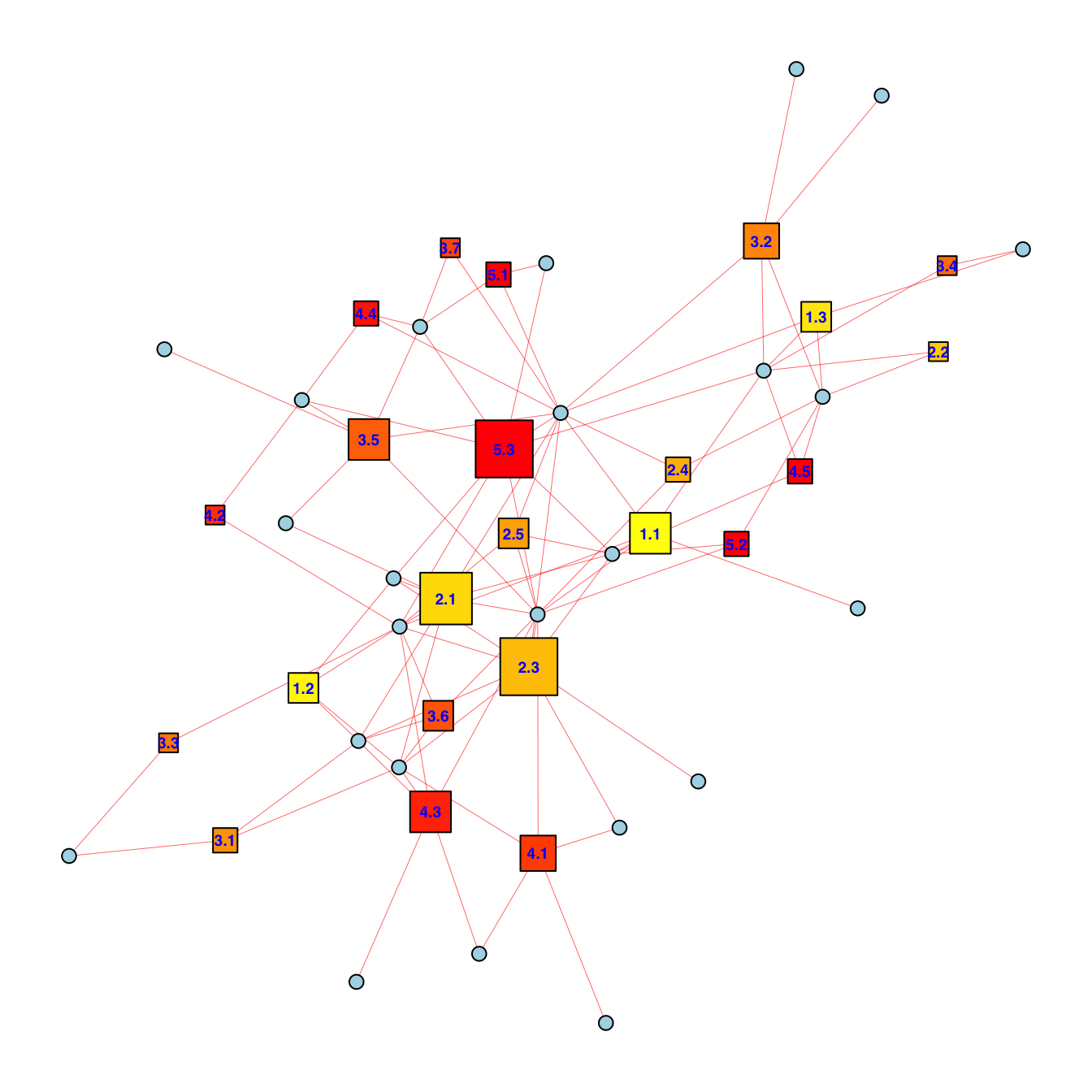
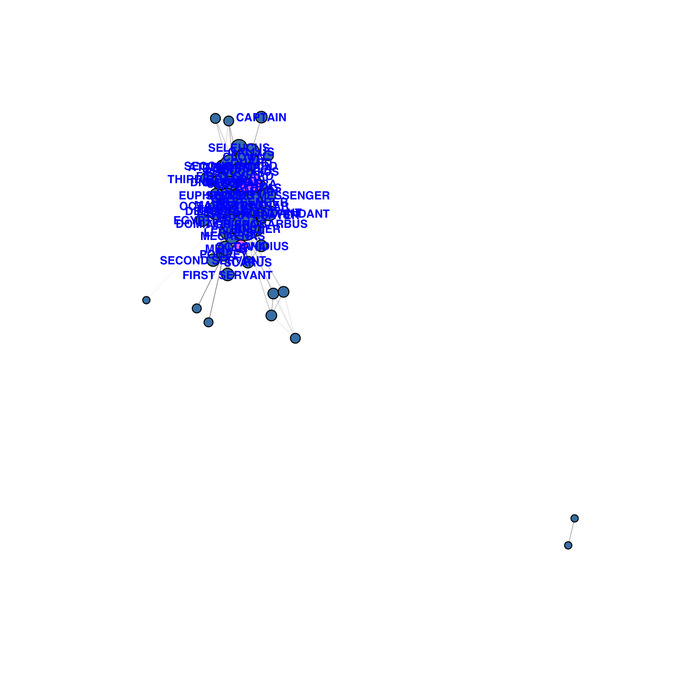
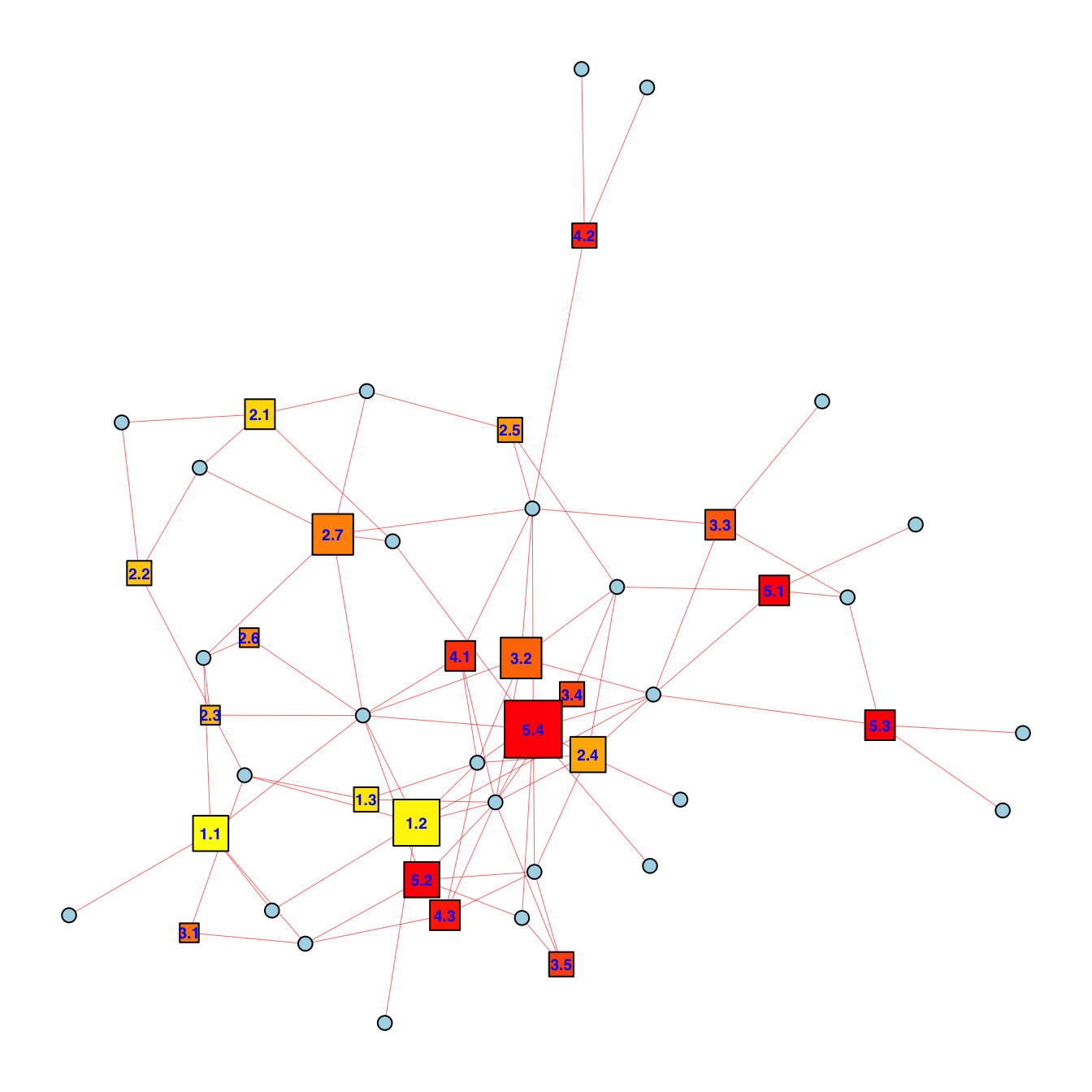
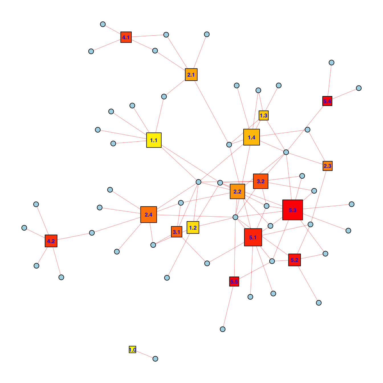
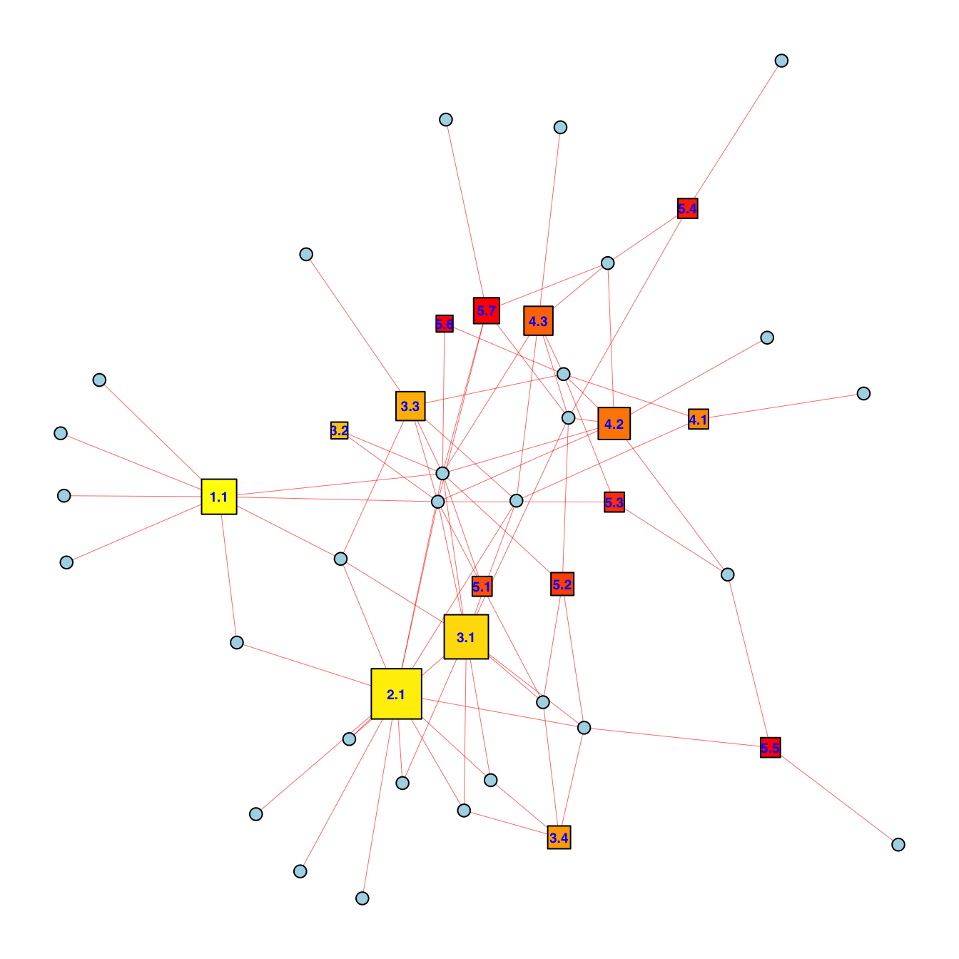
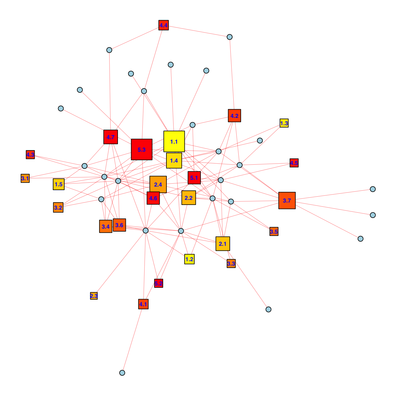
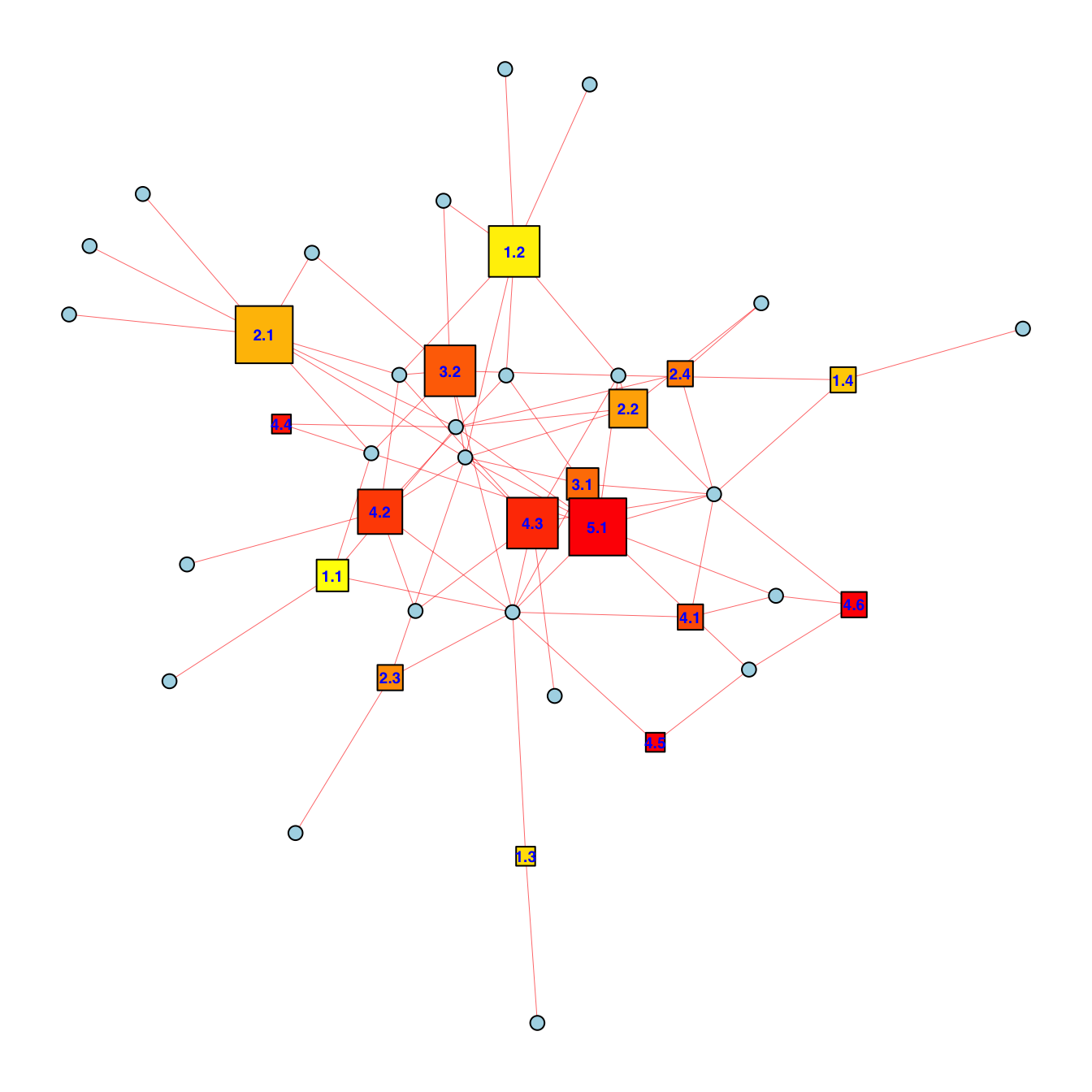
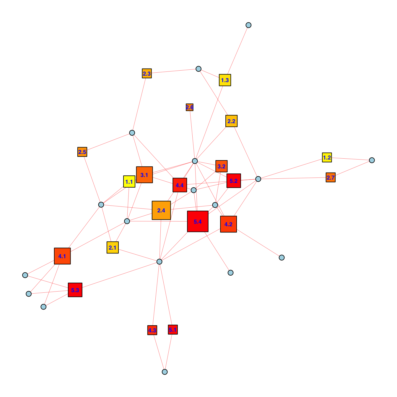
```{r all-network}
#| label: fig-all-netz
#| echo: false
#| message: false
#| warning: false
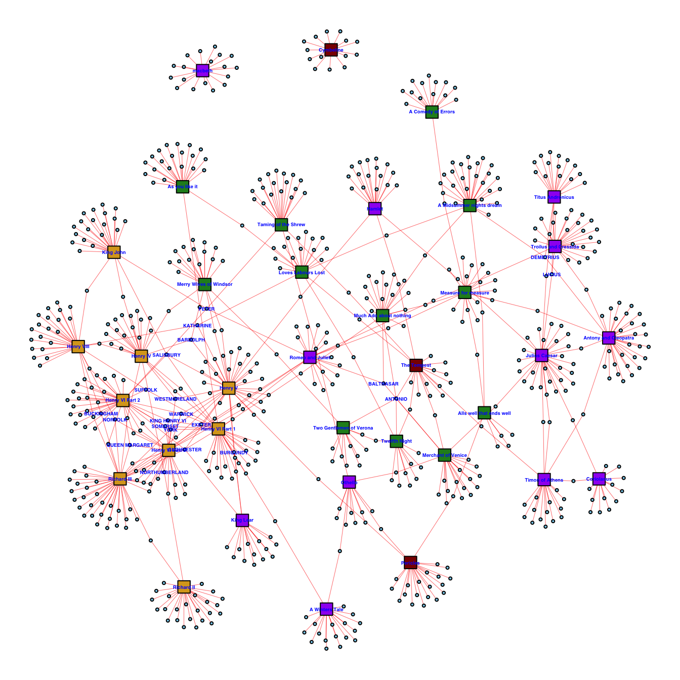
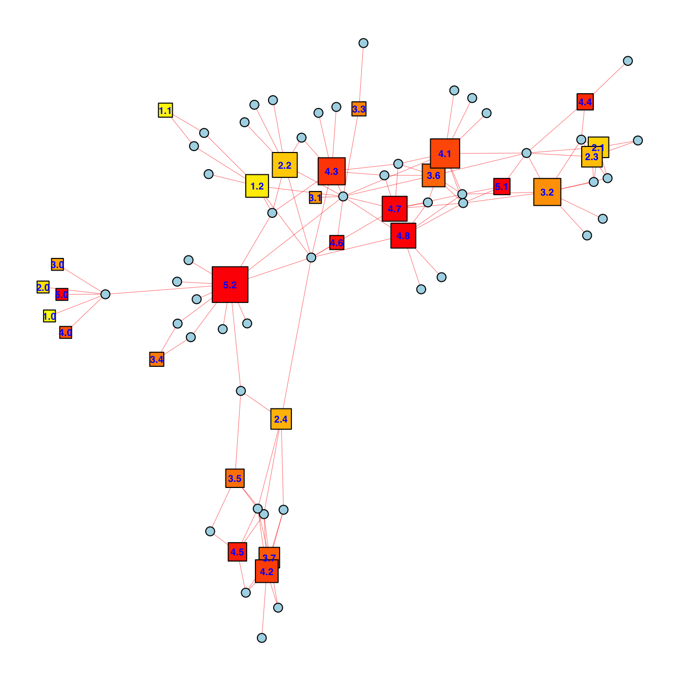
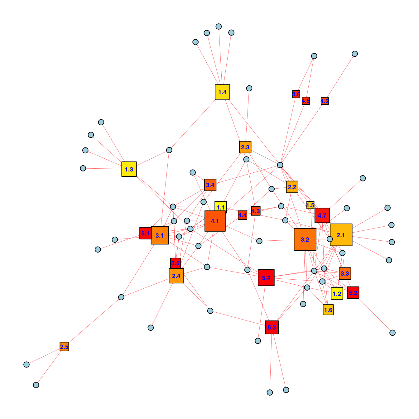
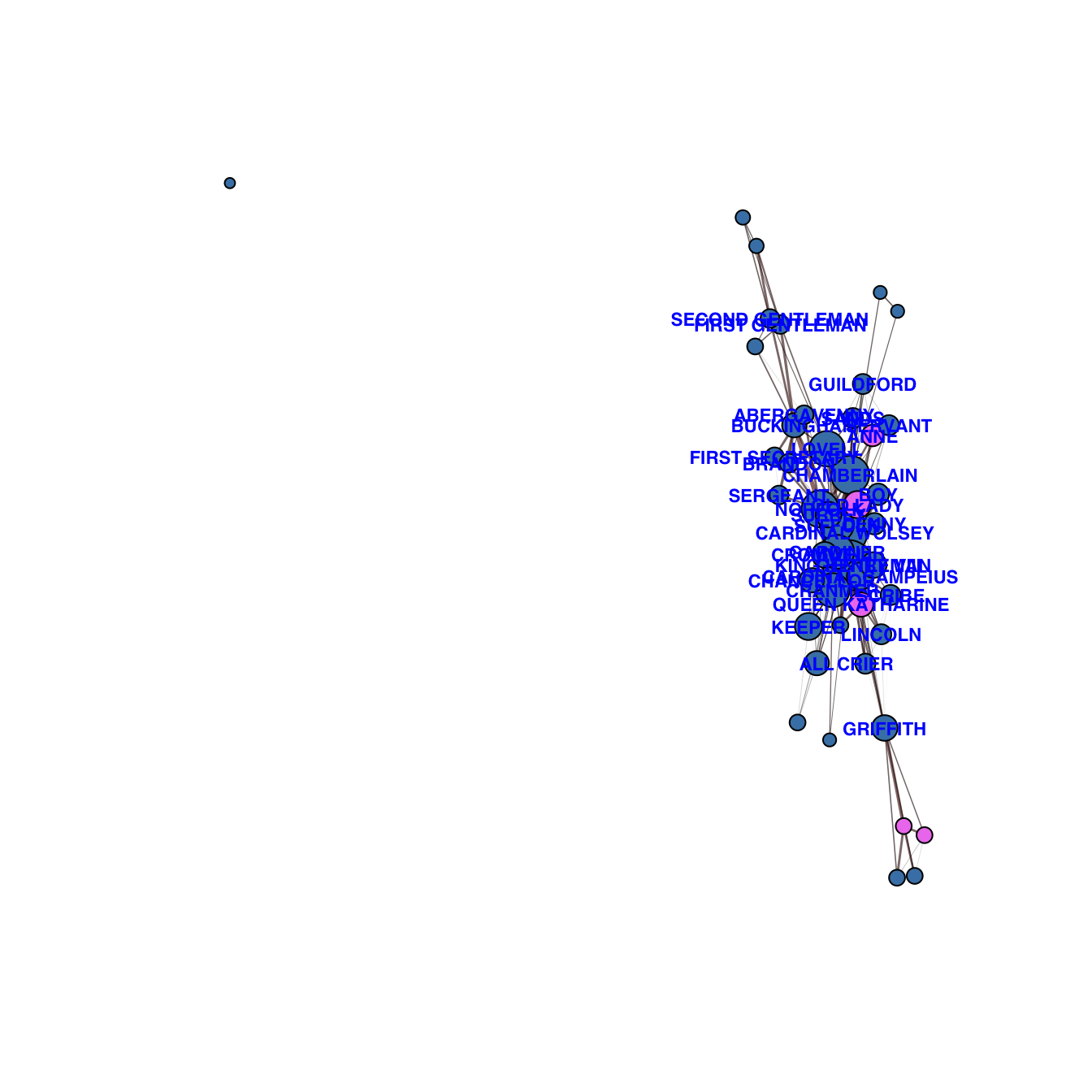
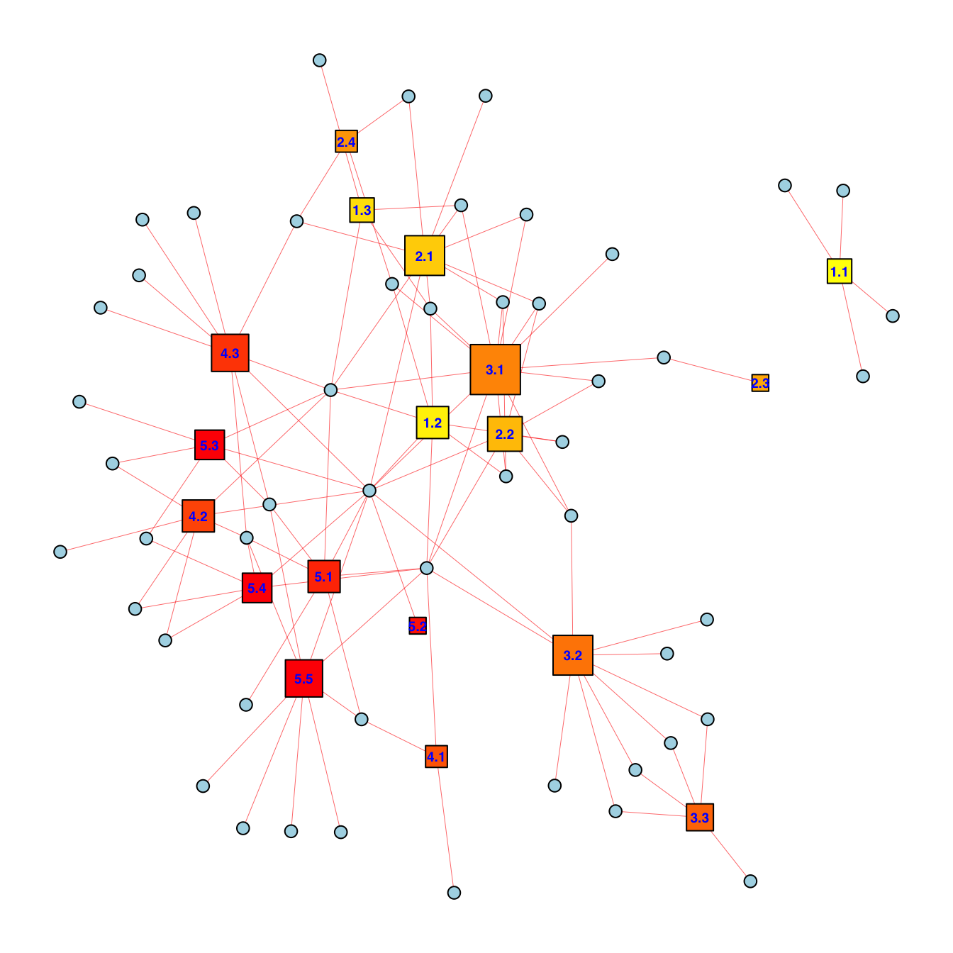
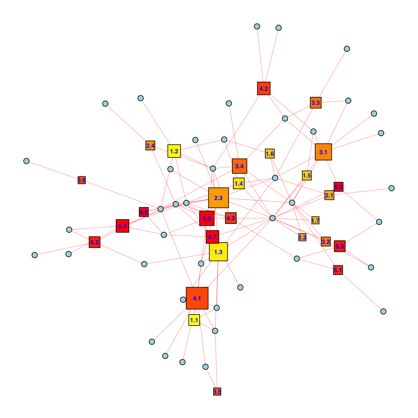
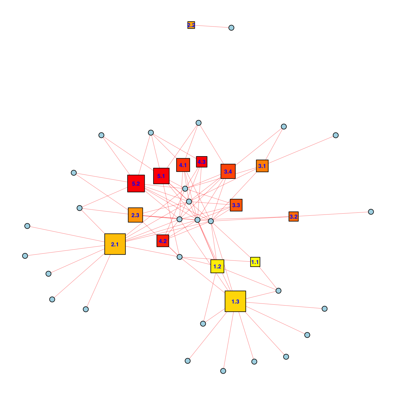
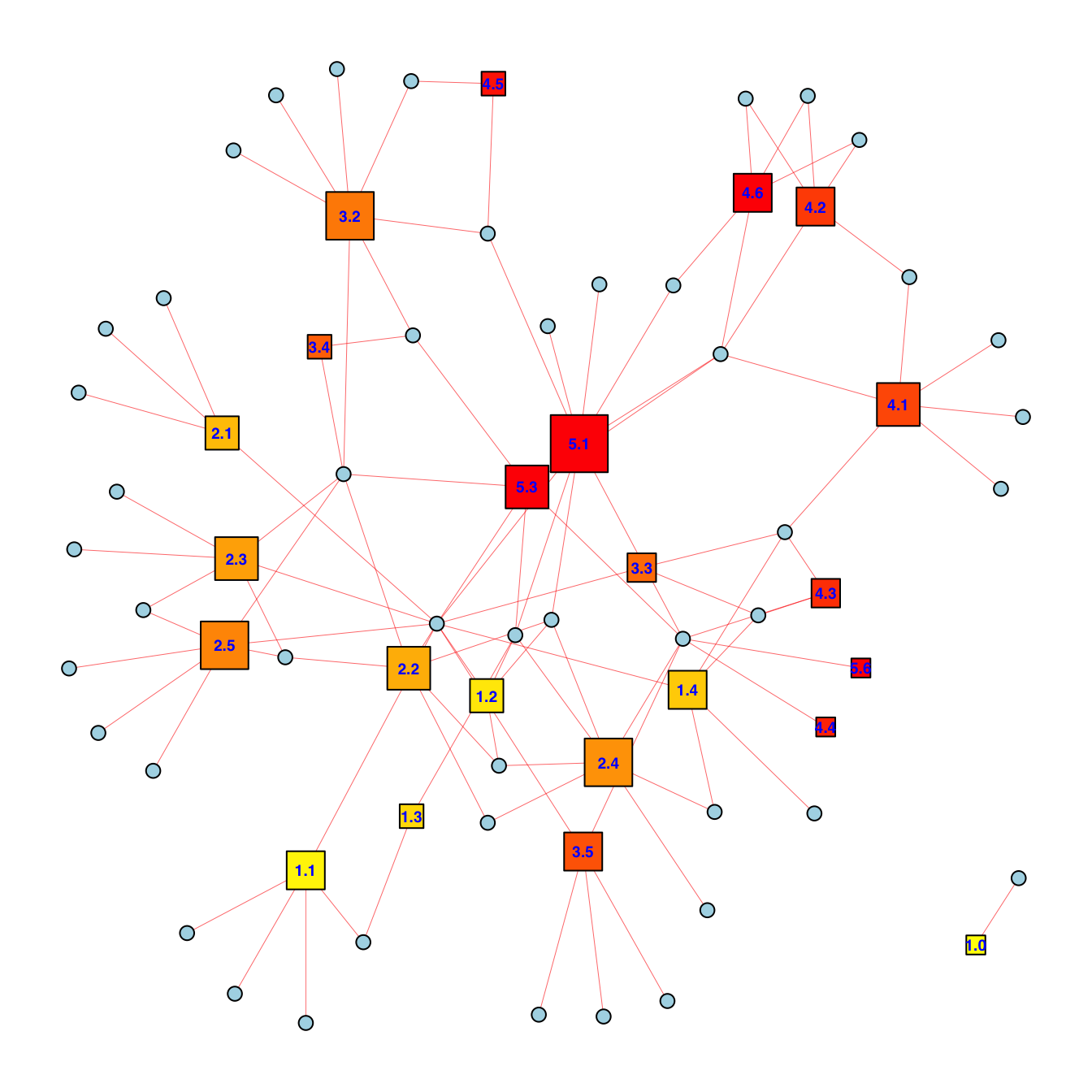
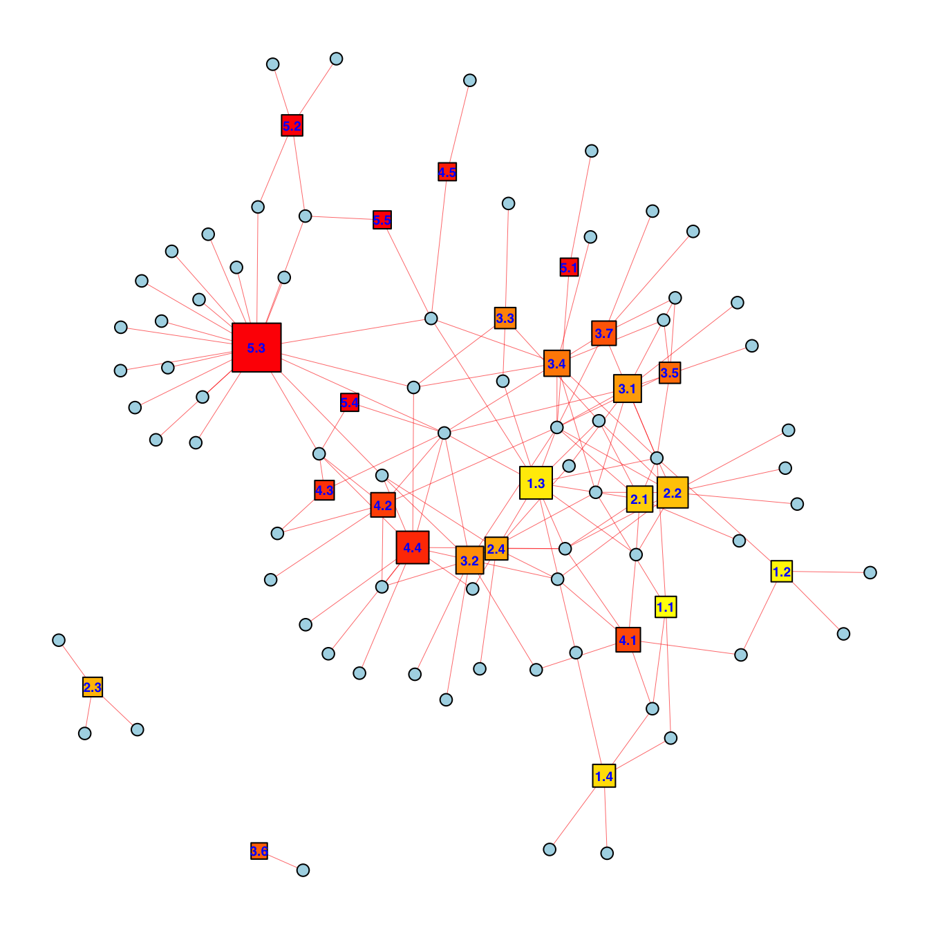
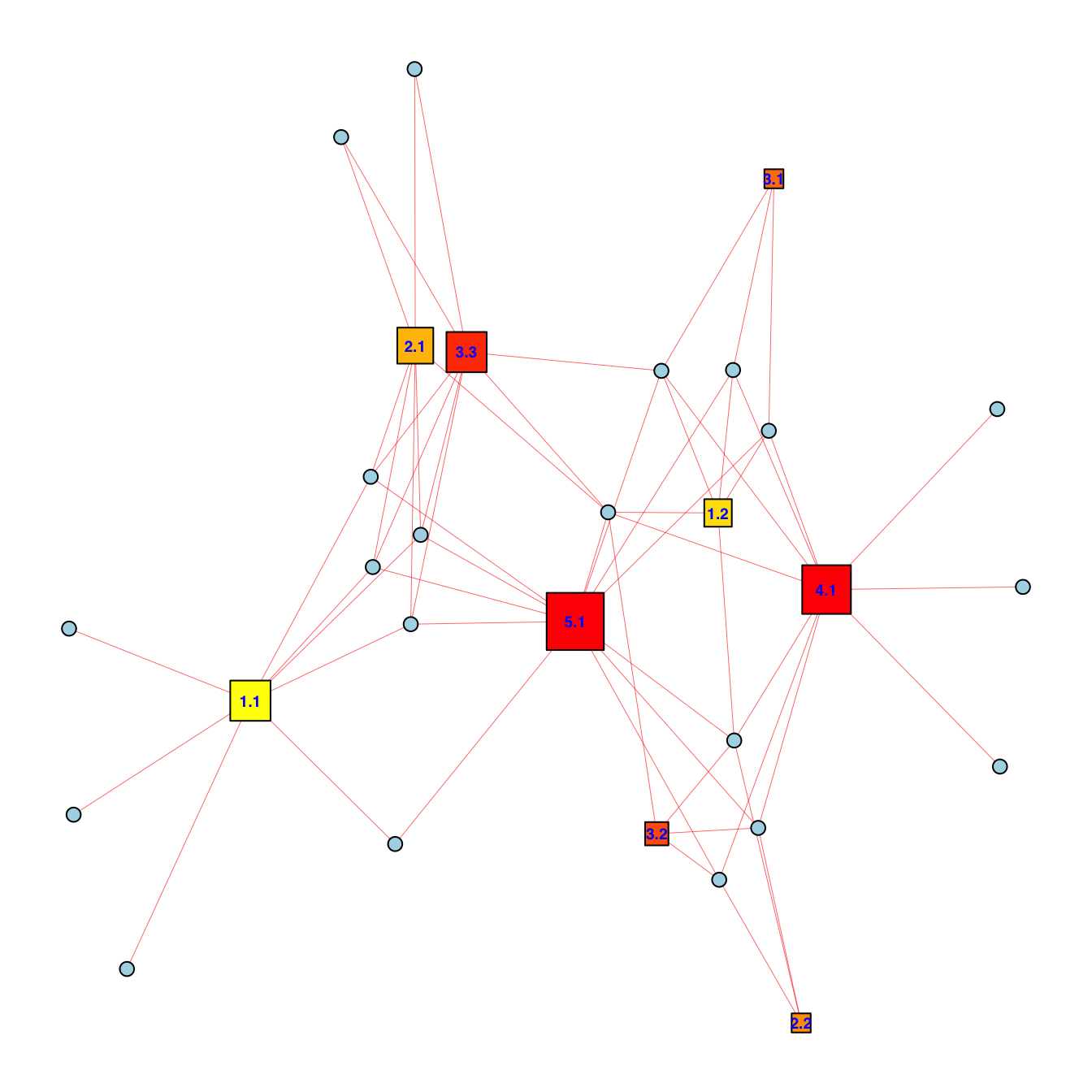
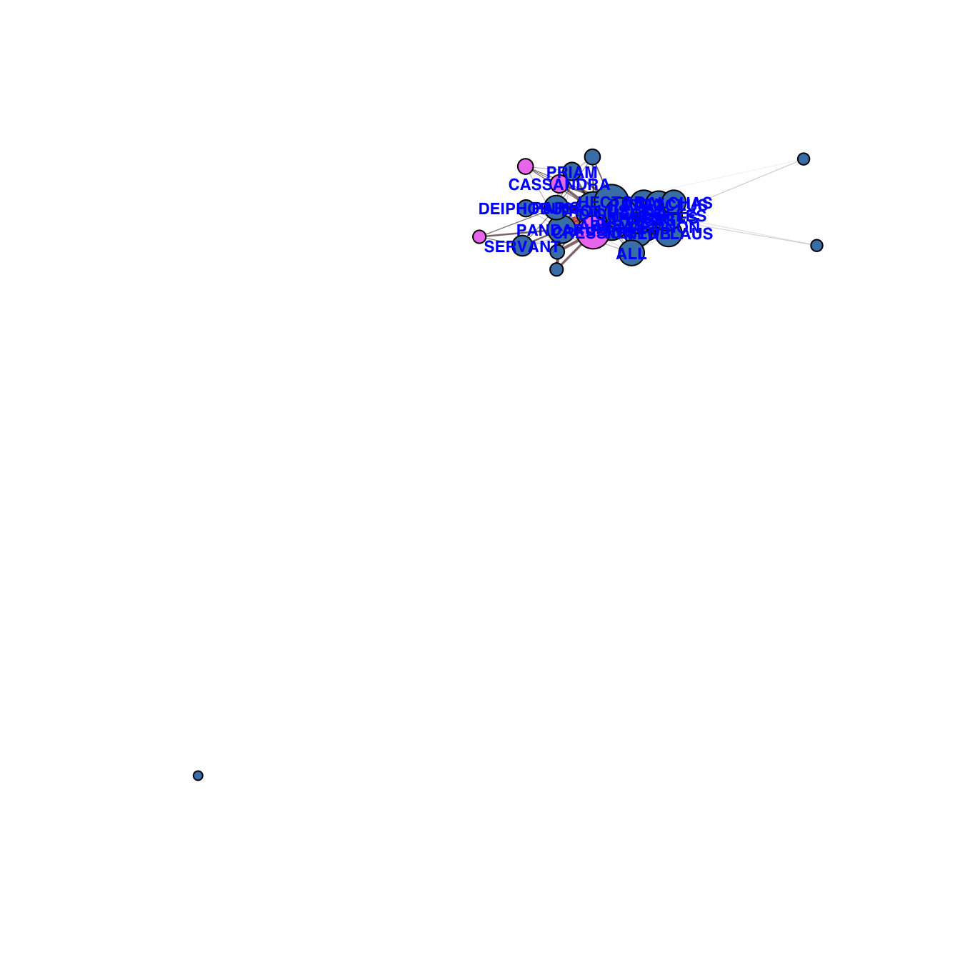
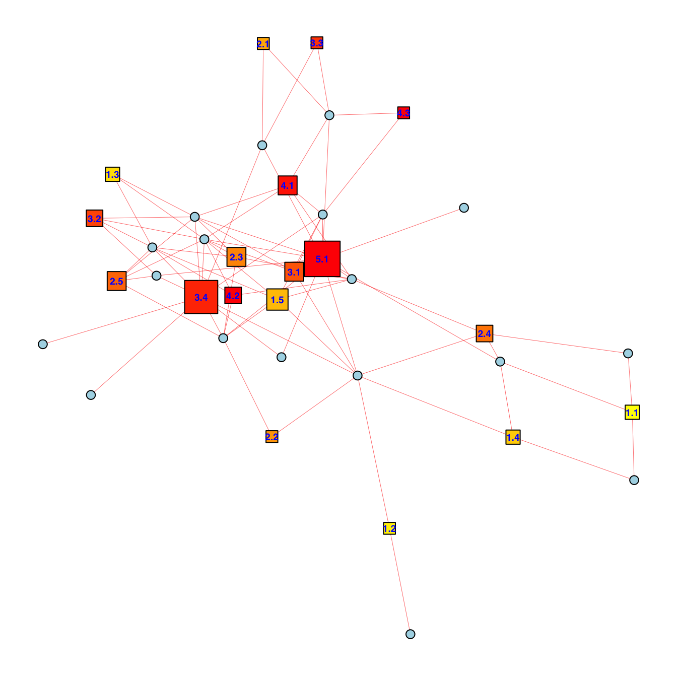
#| fig-cap: Two-mode network of plays and their (named) characters. Naturally, the history plays share the most number of characters.
#| paged-print: false
#| fig.height: 7
library(igraph)
## two mode with plays as squares and players as circles
shakes_overview_network <- shakes %>%
filter(!is.na(PlayerClean), PlayerClean != "",
!is.na(Scene)) %>% # !is.na(ActSceneLine), ActSceneLine != ""
select(Play, PlayerClean) %>%
distinct()
unnamed <- c("FIRST CARRIER", "OSTLER", "SECOND CARRIER", "FIRST TRAVELLER", "THIEVES", "SERVANT", "VINTNER", "HOSTESS", "SHERIFF", "CARRIER", "MESSENGER", "FIRST WARDER", "SECOND WARDER", "MAYOR", "OFFICER", "BOY", "SERGEANT", "FIRST SENTINEL", "SENTINELS", "SOLDIER", "CAPTAIN", "PORTER", "LAWYER", "FIRST GAOLER", "ALL", "FIRST SOLDIER", "WATCH", "GENERAL", "LEGATE", "SCOUT", "CARDINAL", "FIRST PETITIONER", "SECOND PETITIONER", "SPIRIT", "TOWNSMAN", "WIFE", "BOTH", "FIRST NEIGHBOUR", "SECOND NEIGHBOUR", "THIRD NEIGHBOUR", "SERVANTS", "HERALD", "POST", "FIRST MURDERER", "SECOND MURDERER", "FIRST MURDER", "COMMONS", "FIRST GENTLEMAN", "SECOND GENTLEMAN", "MASTER", "CLERK", "FIRST CITIZEN", "SON", "FATHER", "FIRST KEEPER", "SECOND KEEPER", "NOBLEMAN", "FIRST WATCHMAN", "SECOND WATCHMAN", "THIRD WATCHMAN", "HUNTSMAN", "LIEUTENANT", "FIRST MESSENGER", "SECOND MESSENGER", "PAGE", "KING", "FIRST LORD", "SECOND LORD", "STEWARD", "FOURTH LORD", "CLOWN", "DUKE", "WIDOW", "SECOND SOLDIER", "GENTLEMAN", "A LORD", "FIRST PAGE", "SECOND PAGE", "ATTENDANT", "SOOTHSAYER", "FIRST ATTENDANT", "SECOND ATTENDANT", "ATTENDANTS", "FIRST SERVANT", "SECOND SERVANT", "THIRD SOLDIER", "FOURTH SOLDIER", "FIRST GUARD", "SECOND GUARD", "THIRD GUARD", "EGYPTIAN", "GUARD", "GAOLER", "FIRST MERCHANT", "SECOND MERCHANT", "SECOND CITIZEN", "FIRST SENATOR", "SECOND SENATOR", "GENTLEWOMAN", "FIRST ROMAN", "SECOND ROMAN", "THIRD ROMAN", "FIRST OFFICER", "SECOND OFFICER", "SENATORS", "THIRD CITIZEN", "FOURTH CITIZEN", "FIFTH CITIZEN", "BOTH CITIZENS", "SIXTH CITIZEN", "ALL CITIZENS", "CITIZENS", "AEDILE", "A PATRICIAN", "SECOND PATRICIAN", "BOTH TRIBUNES", "ROMAN", "VOLSCE", "CITIZEN", "FIRST SERVINGMAN", "SECOND SERVINGMAN", "THIRD SERVINGMAN", "FIRST CONSPIRATOR", "SECOND CONSPIRATOR", "THIRD CONSPIRATOR", "ALL THE LORDS", "LORDS", "ALL CONSPIRATORS", "ALL THE PEOPLE", "THIRD LORD", "QUEEN", "LADY", "FRENCHMAN", "FIRST LADY", "FIRST TRIBUNE", "LORD", "FIRST CAPTAIN", "SECOND CAPTAIN", "SECOND GAOLER", "MOTHER", "FIRST BROTHER", "SECOND BROTHER", "FIRST PLAYER", "PROLOGUE", "PLAYER KING", "PLAYER QUEEN", "FIRST SAILOR", "FIRST CLOWN", "SECOND CLOWN", "FIRST PRIEST", "FIRST AMBASSADOR", "CHORUS", "FRENCH SOLDIER", "SURVEYOR", "OLD LADY", "SCRIBE", "CRIER", "THIRD GENTLEMAN", "KEEPER", "CHANCELLOR", "MAN", "BASTARD", "FRENCH HERALD", "ENGLISH HERALD", "FIRST EXECUTIONER", "FIRST COMMONER", "SECOND COMMONER", "SEVERAL CITIZENS", "POET", "FOOL", "OLD MAN", "THIRD SERVANT", "DOCTOR", "FIRST WITCH", "SECOND WITCH", "THIRD WITCH", "BOTH MURDERERS", "THIRD MURDERER", "FIRST APPARITION", "SECOND APPARITION", "THIRD APPARITION", "SOLDIERS", "SAILOR", "SENATOR", "FOURTH GENTLEMAN", "SECOND GENTLEMEN", "FIRST MUSICIAN", "DAUGHTER", "FIRST FISHERMAN", "SECOND FISHERMAN", "THIRD FISHERMAN", "FIRST KNIGHT", "SECOND KNIGHT", "THIRD KNIGHT", "SECOND SAILOR", "MARSHAL", "KNIGHTS", "FIRST PIRATE", "SECOND PIRATE", "THIRD PIRATE", "FIRST HERALD", "SECOND HERALD", "GENTLEMEN", "GIRL", "CHILDREN", "PRIEST", "ANOTHER", "SCRIVENER", "THIRD MESSENGER", "FOURTH MESSENGER", "NURSE", "SECOND MUSICIAN", "MUSICIAN", "THIRD MUSICIAN", "APOTHECARY", "FIRST HUNTSMAN", "SECOND HUNTSMAN", "PLAYERS", "A PLAYER", "PEDANT", "HABERDASHER", "TAILOR", "MARINERS", "PAINTER", "JEWELLER", "OLD ATHENIAN", "ALL LADIES", "ALL LORDS", "ALL SERVANTS", "FIRST STRANGER", "SECOND STRANGER", "THIRD STRANGER", "THIRD SENATOR", "SOME SPEAK", "SOME OTHERS", "FIRST BANDIT", "SECOND BANDIT", "THIRD BANDIT", "BANDITTI", "TRIBUNES","FIRST GOTH", "SECOND GOTH", "THIRD GOTH", "ALL THE GOTHS", "MYRMIDONS", "FIRST OUTLAW", "SECOND OUTLAW", "THIRD OUTLAW", "OUTLAWS", "SECOND LADY", "MARINER", "LORD", "OFFICER", "SHERIFF", "FIRST SERVANT", "SECOND SERVANT", "SOLDIER", "FIRST SOLDIER", "PORTER", "ATTENDANT", "LORDS", "THIRD CITIZEN", "BOTH", "THIRD GENTLEMAN", "SECOND WATCHMAN")
# shakes_overview_2mode = delete_vertices(shakes_overview_2mode, unnamed)
shakes_overview_network <- shakes_overview_network %>%
filter(!PlayerClean %in% unnamed)
shakes_overview_2mode <- graph_from_data_frame(shakes_overview_network, directed=FALSE)
## distinguish node types (for two-mode plotting)
V(shakes_overview_2mode)$type <- V(shakes_overview_2mode)$name %in% shakes_overview_network$Play
V(shakes_overview_2mode)$shape <- ifelse(V(shakes_overview_2mode)$type, "square", "circle")
V(shakes_overview_2mode)$size <- ifelse(V(shakes_overview_2mode)$type, 4, 1)
## colour by play genre
play_genre_lookup <- shakes %>%
select(Play, Play_Genre) %>%
distinct() %>%
filter(!is.na(Play_Genre)) # remove any missing genres
# Assign colors for genres
genre_colors <- c(
"Tragedy" = "purple",
"History" = "goldenrod",
"Comedy" = "forestgreen",
"Romance" = "darkred"
)
# Assign colors to nodes
V(shakes_overview_2mode)$color <- ifelse(
V(shakes_overview_2mode)$type,
genre_colors[play_genre_lookup$Play_Genre[match(V(shakes_overview_2mode)$name, play_genre_lookup$Play)]],
"skyblue" # Player nodes
)
## labels for only the plays
# vertex_labels <- ifelse(V(shakes_overview_2mode)$type == T, V(shakes_overview_2mode)$name, NA)
vertex_labels <- ifelse(
V(shakes_overview_2mode)$type == TRUE |
(V(shakes_overview_2mode)$type == FALSE & igraph::degree(shakes_overview_2mode) > 2),
V(shakes_overview_2mode)$name,
NA
)
par(mar = c(0, 0, 0, 0))
plot(
shakes_overview_2mode,
# vertex.color = ifelse(V(shakes_overview_2mode)$type, "tomato", "skyblue"), ## organisations, events
vertex.color = V(shakes_overview_2mode)$color,
edge.color = "red",
edge.width = 0.3,
vertex.label = vertex_labels,
vertex.label.family="Helvetica",
vertex.label.color=c("blue"),
vertex.label.font=2, # Font: 1plain, 2bold, 3italic, 4bold italic, 5symbol
vertex.label.cex=0.3,
# vertex.size = 6,
layout = layout_with_fr(shakes_overview_2mode)
)
```
```{r verboseness}
#| label: fig-verboseness
#| echo: false
#| message: false
#| warning: false
#| fig-cap: Most loquacious characters... .
#| paged-print: false
#| fig.height: 5
library(ggplot2)
library(ggiraph)
line_counts_shakes <- shakes %>%
group_by(Play, PlayerClean, sex) %>%
summarise(line_count = n(), .groups = "drop") %>%
arrange(Play, desc(line_count)) %>%
slice_max(line_count, n=20) %>%
arrange(line_count) %>%
mutate(PlayerClean = factor(PlayerClean, levels = PlayerClean))
max_lines <- max(line_counts_shakes$line_count)
p <- ggplot(
line_counts_shakes,
aes(
x = PlayerClean,
y = line_count,
fill = sex,
tooltip = paste0(
"Play: ", Play, "\n",
"Lines: ", line_count)
)
) +
geom_col_interactive(show.legend = FALSE) +
coord_flip() +
scale_fill_manual(
values = c(
"male" = "steelblue",
"female" = "violet",
"other" = "grey"
)
) +
scale_y_continuous(breaks = seq(0, max_lines, 200)) +
labs(x = "", y = "Number of Lines") +
theme_bw()
girafe(
ggobj = p,
options = list(
opts_tooltip(css = "background-color:white;
color:black;
padding:5px;
border:1px solid grey;")
)
)
```
<!-- #| fig-cap: Table of the plays of William Shakespeare. -->
```{r reactable}
#| label: tab-react-shakes
#| echo: false
#| message: false
#| warning: false
#| paged-print: false
library(igraph)
# <https://albert-rapp.de/posts/29_reactable_germany/29_reactable_germany.html>
library(dplyr)
library(stringr)
## producing summary from dataset~~~~~~~~~~~~
# Lead player, counting how many lines each player has in each play
lead_tbl <- shakes %>%
filter(!is.na(PlayerClean)) %>%
count(Play, PlayerClean, name = "Lines") %>%
group_by(Play) %>%
slice_max(order_by = Lines, n = 1, with_ties = FALSE) %>%
ungroup() %>%
select(Play, Lead = PlayerClean)
play_summary <- shakes %>%
group_by(Play) %>%
summarise(
Genre = first(Play_Genre),
Year = first(Play_Year),
Players = n_distinct(PlayerClean, na.rm = TRUE),
Lines = n(),
#unique locations
Locations = SceneCity %>%
na.omit() %>%
unique() %>%
str_trim() %>%
paste(collapse = "; "),
.groups = "drop"
) %>%
# join lead information
left_join(lead_tbl, by = "Play") %>%
select(Play, Genre, Year, Players, Lines, Lead) # Locations
# network connectedness
library(tidyverse)
library(igraph)
compute_act_network <- function(df_act) {
# get unique players in each scene
edges <- df_act %>%
group_by(Scene) %>%
summarise(players = list(unique(PlayerClean)), .groups = "drop") %>%
# create all pairwise combinations only if length > 1
mutate(pairs = map(players, ~ {
if(length(.x) < 2) return(NULL)
t(combn(.x, 2)) %>% as.data.frame()
})) %>%
select(pairs) %>%
unnest(pairs, keep_empty = TRUE)
# If no edges, return NA
if(nrow(edges) == 0) return(NA_real_)
colnames(edges) <- c("from", "to")
# Build igraph object
g <- graph_from_data_frame(edges, directed = FALSE)
# Compute network density using igraph function -- yields measures over 1 because of multiple scene coappearances
igraph::graph.density(g)
}
#network connectedness for each Play and Act
network_df <- shakes %>%
group_by(Play, Act) %>%
summarise(NetworkConnectedness = compute_act_network(cur_data()), .groups = "drop")
# network_df
# prep for react table
shakes_tab <- network_df %>%
summarise(connect = list(NetworkConnectedness), .by=Play)
## play images:
img_urls <- c(
# "A Comedy of Errors"
'https://upload.wikimedia.org/wikipedia/commons/7/79/ComedyErrors1.JPG',
# "A Midsummer nights dream"
'https://upload.wikimedia.org/wikipedia/commons/6/60/John_Simmons_-_Titania_sleeping_in_the_moonlight_protected_by_her_fairies.jpg',
# "A Winters Tale"
'https://upload.wikimedia.org/wikipedia/commons/3/3c/Perdita_Anthony_Frederick_Augustus_Sandys.jpg',
# "Alls well that ends well"
'https://upload.wikimedia.org/wikipedia/commons/a/aa/All%27s_Well_That_Ends_Well_Act_V_Scene_iii.jpg',
# "Antony and Cleopatra"
'https://upload.wikimedia.org/wikipedia/commons/4/4a/Edwin_Austin_Abbey_Cleopatra_Sooth%2C_la%2C_I%E2%80%99ll_Help_Thus_it_must_be_Act_IV%2C_Scene_IV%2C_Antony_and_Cleopatra_1909.jpg',
# "As you like it"
'https://upload.wikimedia.org/wikipedia/commons/5/55/Plate_9%2C_Rosalind_%28R._W._Macbeth%29_12000px.jpg',
# "Coriolanus"
'https://upload.wikimedia.org/wikipedia/commons/8/84/Thomas_Lawrence_-_John_Philip_Kemble_as_Coriolanus_%281798%29.jpg',
# "Cymbeline"
'https://upload.wikimedia.org/wikipedia/commons/9/99/Souchon1872ImogenCymbeline.jpg',
# "Hamlet"
'https://upload.wikimedia.org/wikipedia/commons/6/6a/Edwin_Booth_Hamlet_1870.jpg',
# "Henry IV"
'https://upload.wikimedia.org/wikipedia/commons/2/22/%27Henry_IV%27%2C_Part_I%2C_Act_V%2C_Scene_4%2C_Falstaff_and_the_Dead_Body_of_Hotspur_Robert_Smirke_%281753%E2%80%931845%29_Royal_Shakespeare_Theatre.jpg',
# "Henry V"
'https://upload.wikimedia.org/wikipedia/commons/7/7f/Henry5.JPG',
# "Henry VI Part 1"
'https://upload.wikimedia.org/wikipedia/commons/8/82/Henry_Arthur_Payne_-_Plucking_the_Red_and_White_Roses_in_the_Old_Temple_Gardens.jpg',
# "Henry VI Part 2"
'https://upload.wikimedia.org/wikipedia/commons/3/35/Edwin_Austin_Abbey_-_King_Henry_VI%2C_Part_II%2C_%E2%80%9CCome_hither%2C_gracious_sovereign%2C_view_this_body.%E2%80%9D_%28Act_III%2C_Scene_ii%29_-_1937.1187_-_Yale_University_Art_Gallery.jpg',
# "Henry VI Part 3"
'https://upload.wikimedia.org/wikipedia/commons/5/5e/%27The_Murder_of_Rutland_by_Lord_Clifford%27_by_Charles_Robert_Leslie%2C_1815.JPG',
# "Henry VIII"
'https://upload.wikimedia.org/wikipedia/commons/f/f9/After_Hans_Holbein_the_Younger_-_Portrait_of_Henry_VIII_-_Google_Art_Project.jpg',
# "Julius Caesar"
'https://upload.wikimedia.org/wikipedia/commons/a/ab/Edwin_Austin_Abbey_-_Within_the_Tent_of_Brutus%2C_Enter_the_Ghost_of_Caesar%2C_Julius_Caesar%2C_Act_IV%2C_Scene_III_-_1937.1148_-_Yale_University_Art_Gallery.jpg',
# "King John"
'https://upload.wikimedia.org/wikipedia/commons/8/8a/Herbert_Beerbohm_Tree_%281852%E2%80%931917%29%2C_as_King_John_in_%27King_John%27_by_William_Shakespeare_Charles_A._Buchel_%281872%E2%80%931950%29_Victoria_and_Albert_Museum.jpg',
# "King Lear"
'https://upload.wikimedia.org/wikipedia/commons/3/31/Cordelia%27s_Portion.jpg',
# "Loves Labours Lost"
'https://upload.wikimedia.org/wikipedia/commons/7/7b/%22Love%27s_Labour%27s_Lost%22%2C_Act_IV%2C_Scene_3.jpg',
# "Measure for measure"
'https://upload.wikimedia.org/wikipedia/commons/c/ce/John_Philip_Kemble_%281757%E2%80%931823%29%2C_as_Vicentio_in_%27Measure_for_Measure%27_by_William_Shakespeare%2C_1794_British_School_Victoria_and_Albert_Museum.jpg',
# "Merchant of Venice"
'https://upload.wikimedia.org/wikipedia/commons/b/b3/Portia_and_Shylock_%28Sully%2C_1835%29.jpg',
# "Merry Wives of Windsor"
'https://upload.wikimedia.org/wikipedia/commons/4/40/Falstaff_Wooing_Mistress_Ford.jpg',
# "Much Ado about nothing"
'https://upload.wikimedia.org/wikipedia/commons/b/b7/Shakespeare%27s_Heroines_-_Beatrice.jpg',
# "Othello"
'https://upload.wikimedia.org/wikipedia/commons/4/4b/Othello_et_Desd%C3%A9mone_%C3%A0_Venise_-_Th%C3%A9odore_Chass%C3%A9riau_-_Mus%C3%A9e_du_Louvre_Peintures_RF_3897.jpg',
# "Pericles"
'https://upload.wikimedia.org/wikipedia/commons/8/8c/Marina_singing_before_Pericles_%28Stothard%2C_1825%29.jpg',
# "Richard II"
'https://upload.wikimedia.org/wikipedia/commons/a/a7/The_Entry_of_Richard_and_Bolingbroke_into_London_%28from_William_Shakespeare%27s_%27Richard_II%27%2C_Act_V%2C_Scene_2%29_James_Northcote_%281746%E2%80%931831%29_Royal_Albert_Memorial_Museum.jpg',
# "Richard III"
'https://upload.wikimedia.org/wikipedia/commons/2/2e/George_Frederick_Cooke_as_Richard_III_Thomas_Sully.jpg',
# "A Winters Tale"
'https://upload.wikimedia.org/wikipedia/commons/5/55/Romeo_and_juliet_brown.jpg',
# "Taming of the Shrew"
'https://upload.wikimedia.org/wikipedia/commons/a/ae/Katherine_and_Petruchio.jpg',
# "The Tempest"
'https://upload.wikimedia.org/wikipedia/commons/6/6a/William_Hamilton_Prospero_and_Ariel.jpg',
# "Timon of Athens"
'https://upload.wikimedia.org/wikipedia/commons/a/a1/Brooklyn_Museum_-_The_Fugitive_Study_for_Timon_of_Athens_-_Thomas_Couture.jpg',
# "Titus Andronicus"
'https://upload.wikimedia.org/wikipedia/commons/3/33/Titus_-_Gravelot.jpg',
# "Troilus and Cressida"
'https://upload.wikimedia.org/wikipedia/commons/5/55/Portrait_of_a_Lady_in_the_Character_of_Cressida.jpg',
# "Twelfth Night"
'https://upload.wikimedia.org/wikipedia/commons/c/ce/Daniel_Maclise_%281806-1870%29_-_Scene_from_%27Twelfth_Night%27_%28%27Malvolio_and_the_Countess%27%29_-_N00423_-_National_Gallery.jpg',
# "Two Gentlemen of Verona"
'https://upload.wikimedia.org/wikipedia/commons/1/1e/Scene_from_%28Kauffmann%29.jpg',
# "macbeth"
'https://upload.wikimedia.org/wikipedia/commons/a/a5/Macbeth_and_Banquo_with_the_witches_JHF.jpg'
)
shakes_summary <- play_summary %>%
mutate(
img=img_urls,
.before = 1
) %>%
left_join(shakes_tab, by='Play')
shakes_summary$Lead <- str_to_title(shakes_summary$Lead)
shakes_summary$connect <- lapply(shakes_summary$connect, function(x) {
if(length(x) > 5) {
x[1:5]
} else {
x
}
})
connect_means <- shakes_summary$connect %>%
lapply(function(x) {
names(x) <- paste0(seq_along(x))
as_tibble_row(x)
}) %>%
bind_rows() %>%
colMeans(na.rm = TRUE)
bottom_row <- tibble(
img = "https://upload.wikimedia.org/wikipedia/commons/2/21/William_Shakespeare_by_John_Taylor%2C_edited.jpg",
Play = "Shakespeare",
Genre = "All",
Year = 1564,
Players = sum(shakes_summary$Players, na.rm = TRUE),
Lines = sum(shakes_summary$Lines, na.rm = TRUE),
Lead = "Shakespeare",
# Locations = "Stratford-upon-Avon",
connect = list(connect_means)
)
shakes_summary_w_bottom <- bind_rows(shakes_summary, bottom_row)
# short play descriptions
play_desc <- c(
# "A Comedy of Errors"
'Set in the Greek city of Ephesus, The Comedy of Errors tells the story of two sets of identical twins who were accidentally separated at birth. Antipholus of Syracuse and his servant, Dromio of Syracuse, arrive in Ephesus, which turns out to be the home of their twin brothers, Antipholus of Ephesus and his servant, Dromio of Ephesus. When the Syracusans encounter the friends and families of their twins, a series of wild mishaps based on mistaken identities lead to wrongful beatings, a near-seduction, the arrest of Antipholus of Ephesus, and false accusations of infidelity, theft, madness, and demonic possession.',
# "A Midsummer nights dream"
'The play is set in Athens, and consists of several subplots that revolve around the marriage of Theseus and Hippolyta. One subplot involves a conflict among four Athenian lovers. Another follows a group of six amateur actors rehearsing the play which they are to perform before the wedding. Both groups find themselves in a forest inhabited by fairies who manipulate the humans and are engaged in their own domestic intrigue.',
# "A Winters Tale"
'King Leontes’ jealousy leads him to wrongly accuse his wife of infidelity, causing tragedy. Years later, redemption, reconciliation, and miraculous reunions restore hope and family bonds.',
# "Alls well that ends well"
'Helena cures the King of France’s illness and pursues her love, Bertram, through clever schemes. Challenges, misunderstandings, and social constraints are overcome, emphasizing perseverance and wit.',
# "Antony and Cleopatra"
'The plot is based on Thomas North\'s 1579 English translation of Plutarch\'s Lives (in Ancient Greek) and follows the relationship between Cleopatra and Mark Antony from the time of the Sicilian revolt to Cleopatra\'s suicide during the War of Actium. The main antagonist is Octavius Caesar, one of Antony\'s fellow triumvirs of the Second Triumvirate and the first emperor of the Roman Empire. The tragedy is mainly set in the Roman Republic and Ptolemaic Egypt and is characterized by swift shifts in geographical location and linguistic register as it alternates between sensual, imaginative Alexandria and a more pragmatic, austere Rome.',
# "As you like it"
'As You Like It follows its heroine Rosalind as she flees persecution in her uncle\'s court, accompanied by her cousin Celia to find safety and, eventually, love, in the Forest of Arden. In the forest, they encounter a variety of memorable characters, notably the melancholy traveller Jaques, who speaks one of Shakespeare\'s most famous speeches ("All the world\'s a stage") and provides a sharp contrast to the other characters in the play, always observing and disputing the hardships of life in the country.',
# "Coriolanus"
'Coriolanus is the name given to a Roman general after his military feats against the Volscians at Corioli. Following his success, others encourage Coriolanus to pursue the consulship, but his disdain for the plebeians and mutual hostility with the tribunes lead to his banishment from Rome. In exile, he presents himself to the Volscians, then leads them against Rome. After he relents and agrees to a peace with Rome, he is killed by his previous Volscian allies.',
# "Cymbeline"
'Cymbeline, also known as The Tragedie of Cymbeline or Cymbeline, King of Britain, is a play by William Shakespeare set in Ancient Britain (c.10–14 AD) and based on legends that formed part of the Matter of Britain concerning the early historical Celtic British King Cunobeline.',
# "Hamlet"
'Set in Denmark, the play depicts Prince Hamlet and his attempts to exact revenge against his uncle, Claudius, who has murdered Hamlet\'s father in order to seize his throne and marry Hamlet\'s mother.',
# "Henry IV"
'It was composed in the later years of the reign of Elizabeth I, when questions of succession and political stability were prominent. Set in England in the early 1400s during the reign of Henry IV, the play depicts rebellion against the crown alongside the development of Prince Hal, the future Henry V, and examines themes of leadership and the formation of the heir apparent.',
# "Henry V"
'It tells the story of King Henry V of England, focusing on events immediately before and after the Battle of Agincourt (1415) during the Hundred Years\' War. In the First Quarto text, it was titled The Cronicle History of Henry the fift and The Life of Henry the Fifth in the First Folio text.',
# "Henry VI Part 1"
'Henry VI, Part 1 deals with the loss of England\'s French territories and the political machinations leading up to the Wars of the Roses, as the English political system is torn apart by personal squabbles and petty jealousy. Henry VI, Part 2 deals with the King\'s inability to quell the bickering of his nobles and the inevitability of armed conflict and Henry VI, Part 3 deals with the horrors of that conflict.',
# "Henry VI Part 2"
'Henry VI, Part 2 (1591) is a Shakespearean history play about King Henry VI of England\'s inability to quell the bickering of his noblemen, the death of his trusted advisor Humphrey, Duke of Gloucester, and the political rise of Richard of York, 3rd Duke of York; it culminates with the First Battle of St Albans (1455), the initial battle of the Wars of the Roses, which were civil wars between the House of Lancaster and the House of York.',
# "Henry VI Part 3"
'Whereas 1 Henry VI deals with the loss of England\'s French territories and the political machinations leading up to the Wars of the Roses and 2 Henry VI focuses on the King\'s inability to quell the bickering of his nobles, and the inevitability of armed conflict, 3 Henry VI deals primarily with the horrors of that conflict, with the once stable nation thrown into chaos and barbarism as families break down and moral codes are subverted in the pursuit of revenge and power.',
# "Henry VIII"
'The Famous History of the Life of King Henry the Eighth, often shortened to Henry VIII, is a collaborative history play, written by William Shakespeare and John Fletcher, based on the life of Henry VIII. An alternative title, All Is True, is recorded in contemporary documents, with the title Henry VIII not appearing until the play\'s publication in the First Folio of 1623.',
# "Julius Caesar"
'The play portrays the political conspiracy that led to the assassination of the Roman dictator Julius Caesar and Rome\'s subsequent civil war. Drawing primarily (with deviations in various aspects) from Sir Thomas North\'s 1579 translation of Parallel Lives by Plutarch, Shakespeare presents a dramatised account of Caesar\'s growing power, his murder by a group of senators led by Cassius and Brutus, and the defeat of the conspirators by the forces of Mark Antony and Octavius at the Battle of Philippi.',
# "King John"
'The Life and Death of King John (also King John) is a history play about the reign of John, King of England (r. 1199–1216), the son of Henry II and Eleanor of Aquitaine, and the father of Henry III.',
# "King Lear"
'Set in pre-Roman Britain, the play depicts the consequences of King Lear\'s love-test, in which he divides his power and land according to the praise of his daughters. The play is known for its dark tone, complex poetry, and prominent motifs concerning blindness, madness and human nature.',
# "Loves Labours Lost"
'It follows the King of Navarre and his three companions as they attempt to swear off the company of women for three years in order to focus on study and fasting. Their subsequent infatuation with the Princess of France and her ladies makes them forsworn (break their oath). In an untraditional ending for a comedy, the play closes with the death of the Princess\'s father, and all weddings are delayed for a year. The play draws on themes of masculine love and desire, reckoning and rationalisation, and reality versus fantasy.',
# "Measure for measure"
'The play centres on the despotic and puritan Angelo, a deputy entrusted to rule the city of Vienna in the absence of Duke Vincentio, who instead disguises himself as a humble friar to observe Angelos regency and the lives of his citizens. Angelo persecutes a young man, Claudio, for the crime of fornication, sentencing him to death on a technicality. Angelo then attempts to exploit Isabella (the sister of Claudio), a chaste and innocent nun, when she comes to plead for the life of her brother.',
# "Merchant of Venice"
'A merchant in Venice named Antonio defaults on a large loan taken out on behalf of his dear friend, Bassanio, and provided by a Jewish moneylender, Shylock, with seemingly inevitable fatal consequences.',
# "Merry Wives of Windsor"
'It features the character Sir John Falstaff, the fat knight who had previously been featured in Henry IV, Part 1 and Part 2. Tradition has it that The Merry Wives of Windsor was written at the request of Queen Elizabeth I, who watching Henry IV, Part 1, is said to have asked Shakespeare to write a play depicting Falstaff in love.',
# "Much Ado about nothing"
'The play is set in Messina and revolves around two romantic pairings that emerge when a group of soldiers arrive in the town. The first, between Claudio and Hero, is nearly scuppered by the accusations of the villain, Don John. The second, between Benedick and Beatrice, takes centre stage as the play continues, with their wit and banter providing much of the humour.',
# "Othello"
'Set in Venice and Cyprus, the play depicts the Moorish military commander Othello as he is manipulated by his ensign, Iago, into suspecting his wife Desdemona of infidelity. Othello is widely considered one of Shakespeares greatest works and is usually classified among his major tragedies alongside Macbeth, King Lear, and Hamlet.',
# "Pericles"
'Pericles undergoes perilous adventures, shipwrecks, and family separation. His journey culminates in reunion, restoration, and the triumph of endurance and providence.',
# "Richard II"
'The Tragedy of Richard the Third, often shortened to Richard III, is a play by William Shakespeare, which depicts the Machiavellian rise to power and subsequent short reign of King Richard III of England.',
# "Richard III"
'Richard manipulates, murders, and schemes to seize the English throne. His cunning ascent is followed by paranoia and downfall, illustrating ambition, deceit, and the fragility of power.',
# "A Winters Tale"
'A Winters Tale belongs to a tradition of tragic romances stretching back to antiquity. The plot is based on an Italian tale written by Matteo Bandello, translated into verse as The Tragical History of Romeus and Juliet by Arthur Brooke in 1562, and retold in prose in Palace of Pleasure by William Painter in 1567. Shakespeare borrowed heavily from both but expanded the plot by developing a number of supporting characters, in particular Mercutio and Paris.',
# "Taming of the Shrew"
'The main plot depicts the courtship of Petruchio and Katherina, the headstrong, obdurate shrew. Initially, Katherina is an unwilling participant in the relationship; however, Petruchio "tames" her with various psychological and physical torments, such as keeping her from eating and drinking, until she becomes a desirable, compliant, and obedient bride. The subplot features a competition among the suitors of Katherinas younger sister, Bianca, who is seen as the "ideal" woman.',
# "The Tempest"
'After the first scene, which takes place on a ship at sea during a storm, the rest of the play is set on a remote island, where Prospero, a magician, lives with his daughter Miranda, and his two servants: Caliban, a savage monster figure, and Ariel, an airy spirit. The play contains music and songs that evoke the spirit of enchantment on the island. It explores many themes, including magic, betrayal, revenge, forgiveness and family. In Act IV, a wedding masque serves as a play-within-a-play, and contributes spectacle, allegory, and elevated language.',
# "Timon of Athens"
'Timon lavishes his wealth on parasitic companions until he is poor and rejected by them. He then denounces all of mankind, and isolates himself in a cave in the wilderness.',
# "Titus Andronicus"
'Titus, a general in the Roman army, presents Tamora, Queen of the Goths, as a slave to the new Roman emperor, Saturninus. Saturninus takes her as his wife. From this position, Tamora vows revenge against Titus for killing her son. Titus and his family retaliate, leading to a cycle of violence.',
# "Troilus and Cressida"
'At Troy during the Trojan War, Troilus and Cressida begin a love affair. Cressida is forced to leave Troy to join her father in the Greek camp. Meanwhile, the Greeks endeavour to lessen the pride of Achilles.',
# "Twelfth Night"
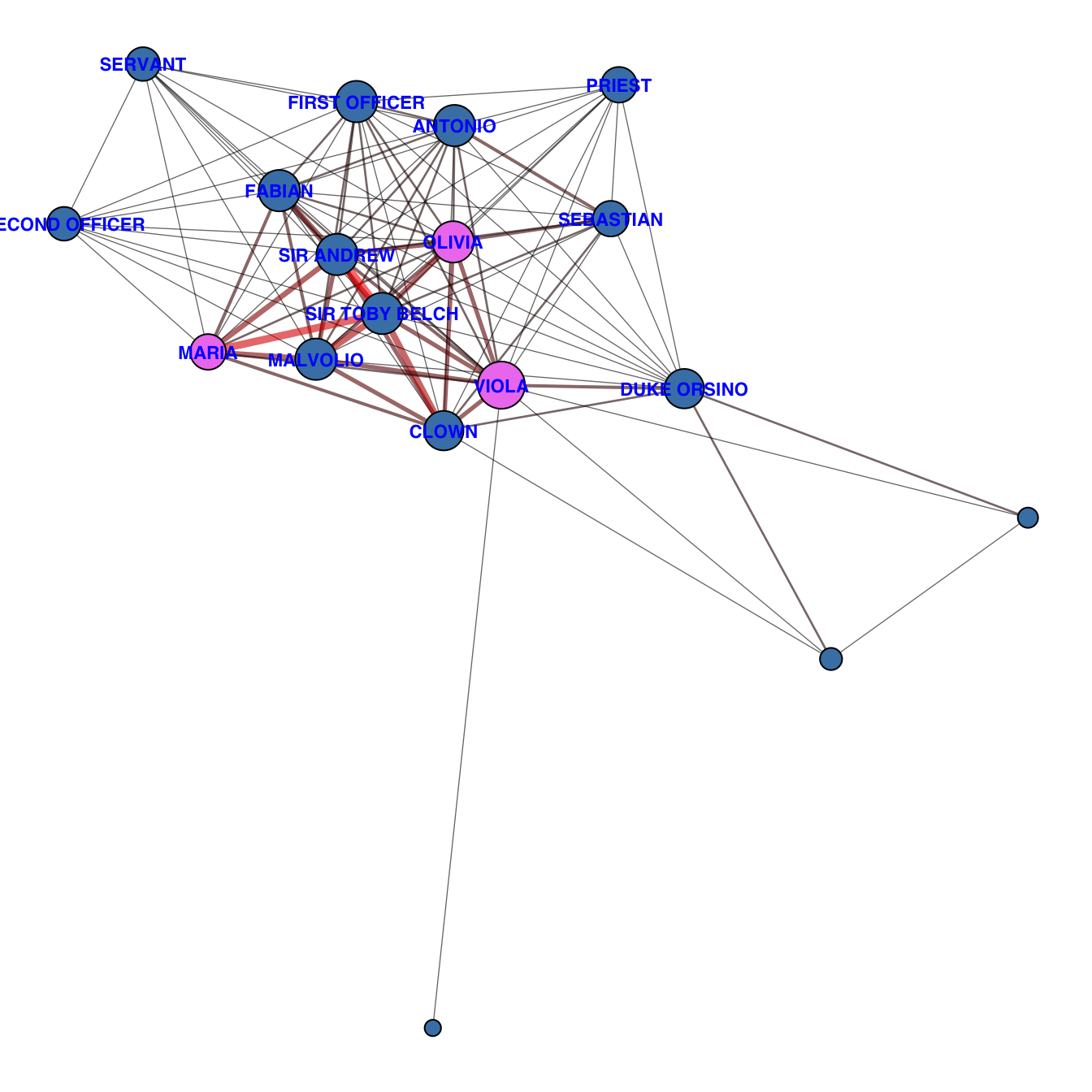
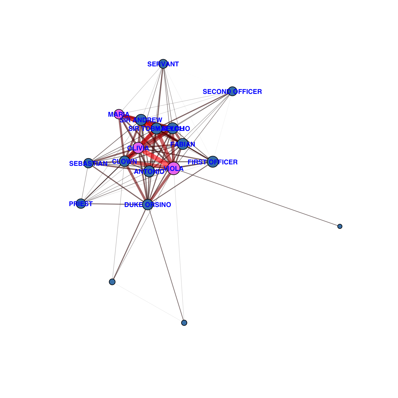
'The play centres on the twins Viola and Sebastian, who are separated in a shipwreck. Viola (disguised as a page named Cesario) falls in love with the Duke Orsino, who in turn is in love with Countess Olivia. Upon meeting Viola, Countess Olivia falls in love with her, thinking she is a man.',
# "Two Gentlemen of Verona"
'The play deals with the themes of friendship and infidelity, the conflict between friendship and love, and the foolish behaviour of people in love. The highlight of the play is considered by some to be Launce, the clownish servant of Proteus, and his dog Crab, to whom "the most scene-stealing non-speaking role in the canon" has been attributed.',
# "macbeth"
'In the play, a brave Scottish general named Macbeth receives a prophecy from a trio of witches that one day he will become King of Scotland. Consumed by his latent ambition and spurred to violence by his wife, Macbeth murders King Duncan and takes the Scottish throne for himself. Then, racked with guilt and paranoia, he commits further murders to protect himself from enmity and suspicion, becoming a tyrannical ruler in the process. The violence perpetrated by the power-hungry couple leads to their insanity and finally to their deaths.'
)
play_urls <- c(
# "A Comedy of Errors"
"https://en.wikipedia.org/wiki/The_Comedy_of_Errors",
# "A Midsummer nights dream"
"https://en.wikipedia.org/wiki/A_Midsummer_Night%27s_Dream",
# "A Winters Tale"
"https://en.wikipedia.org/wiki/The_Winter%27s_Tale",
# "Alls well that ends well"
"https://en.wikipedia.org/wiki/All's_Well_That_Ends_Well",
# "Antony and Cleopatra"
"https://en.wikipedia.org/wiki/Antony_and_Cleopatra",
# "As you like it"
"https://en.wikipedia.org/wiki/As_You_Like_It",
# "Coriolanus"
"https://en.wikipedia.org/wiki/Coriolanus",
# "Cymbeline"
"https://en.wikipedia.org/wiki/Cymbeline",
# "Hamlet"
"https://en.wikipedia.org/wiki/Hamlet",
# "Henry IV"
"https://en.wikipedia.org/wiki/Henry_IV,_Part_1",
# "Henry V"
"https://en.wikipedia.org/wiki/Henry_V_(play)",
# "Henry VI Part 1"
"https://en.wikipedia.org/wiki/Henry_VI,_Part_1",
# "Henry VI Part 2"
"https://en.wikipedia.org/wiki/Henry_VI,_Part_2",
# "Henry VI Part 3"
"https://en.wikipedia.org/wiki/Henry_VI,_Part_3",
# "Henry VIII"
"https://en.wikipedia.org/wiki/Henry_VIII_(play)",
# "Julius Caesar"
"https://en.wikipedia.org/wiki/Julius_Caesar_(play)",
# "King John"
"https://en.wikipedia.org/wiki/King_John_(play)",
# "King Lear"
"https://en.wikipedia.org/wiki/King_Lear",
# "Loves Labours Lost"
"https://en.wikipedia.org/wiki/Love%27s_Labour%27s_Lost",
# "Measure for measure"
"https://en.wikipedia.org/wiki/Measure_for_Measure",
# "Merchant of Venice"
"https://en.wikipedia.org/wiki/The_Merchant_of_Venice",
# "Merry Wives of Windsor"
"https://en.wikipedia.org/wiki/The_Merry_Wives_of_Windsor",
# "Much Ado about nothing"
"https://en.wikipedia.org/wiki/Much_Ado_About_Nothing",
# "Othello"
"https://en.wikipedia.org/wiki/Othello",
# "Pericles"
"https://en.wikipedia.org/wiki/Pericles,_Prince_of_Tyre",
# "Richard II"
"https://en.wikipedia.org/wiki/Richard_II_(play)",
# "Richard III"
"https://en.wikipedia.org/wiki/Richard_III_(play)",
# "A Winters Tale"
"https://en.wikipedia.org/wiki/Romeo_and_Juliet",
# "Taming of the Shrew"
"https://en.wikipedia.org/wiki/The_Taming_of_the_Shrew",
# "The Tempest"
"https://en.wikipedia.org/wiki/The_Tempest",
# "Timon of Athens"
"https://en.wikipedia.org/wiki/Timon_of_Athens",
# "Titus Andronicus"
"https://en.wikipedia.org/wiki/Titus_Andronicus",
# "Troilus and Cressida"
"https://en.wikipedia.org/wiki/Troilus_and_Cressida",
# "Twelfth Night"
"https://en.wikipedia.org/wiki/Twelfth_Night",
# "Two Gentlemen of Verona"
"https://en.wikipedia.org/wiki/The_Two_Gentlemen_of_Verona",
# "macbeth"
"https://en.wikipedia.org/wiki/Macbeth"
)
library(reactable)
library(reactablefmtr)
library(htmltools)
main_color <- '#004225'
library(ggiraph)
spark_line <- function(value, row_index, column_name) {
acts <- 1:5
y_rng <- range(c(0, unlist(shakes_summary_w_bottom$connect)),
na.rm = TRUE)
# Create static ggplot with `value` vector
gg_plt <- ggplot(mapping = aes(x = acts, y = value)) +
geom_ribbon(
aes(
x = acts,
ymin = 0, ## issue here???
ymax = value
),
alpha = 0.1,
fill = main_color
) +
geom_line(linewidth = 2, color = main_color) +
ggiraph::geom_point_interactive(
aes(
tooltip = paste0("Network \n connectedness: ", round(value, 2) )
),
color = main_color,
size = 30, # reduce size for interactive hover
na.rm = TRUE
) +
scale_y_continuous(
expand = expansion(mult = 0.1),
limits = y_rng
)+
theme_void()
girafe(
ggobj = gg_plt,
width_svg = 16,
height = 9,
options = list(
opts_toolbar(saveaspng = FALSE)
)
)
}
# # Example with first row
# spark_line(shakes_summary_w_bottom$connect[[1]], NA, NA)
play_details <- function(row_index, col_name) {
play_name <- shakes_summary_w_bottom[[row_index, 'Play']]
div(
style = htmltools::css(
display = 'grid',
grid_template_columns = '1fr 2fr',
row_gap = '10px',
padding = '5px 50px'
),
div(
## blank for the moment
),
div(
style = css(
font_family = 'Source Sans Pro',
font_size = '1.25rem'
),
span(
a(
# `state_urls` contains URLs to a state's Wiki page
href = play_urls[row_index],
style = css(
color = main_color,
text_decoration = 'none',
font_weight = 600
),
'From Wikipedia: '
),
play_desc[row_index]
)
)
)
}
# # Example with first row
# play_details(1, '') %>% htmltools::browsable()
ShakesTab_withoutTitle <- shakes_summary %>%
reactable(
pagination = FALSE,
style = list(
fontFamily = '"Source Sans Pro", sans-serif',
fontSize = "16px"
),
# Defaults for all columns
defaultColDef = colDef(
vAlign = "center",
align = "left",
headerStyle = htmltools::css(
font_weight = 600,
border_bottom = "2px solid black"
),
footer = function(values, col_name) {
shakes_summary_w_bottom[[37, col_name]]
},
footerStyle = htmltools::css(
font_weight = 600,
border_top = '2px solid black'
)
),
# Per-column customizations
columns = list(
img = colDef(
header = "",
width = 100,
cell = function(value) {
tags$img(
src = value,
width = 60,
style = "border-radius: 4px;"
)
},
footer = function(value) {
tags$img(
src = shakes_summary_w_bottom$img[37],
width = 50
)
},
details = play_details
),
Play = colDef(width = 125),
Genre = colDef(header = "Genre", width = 90),
Year = colDef(header = "Year", width = 60),
Players = colDef(
header = 'Players',
align = 'center',
width = 80 # ,
# cell = bubble_grid(
# shakes_summary %>% select(Players),
# min_value = 1,
# max_value = 10,
# colors = c(
# colorspace::lighten(main_color, 0.9),
# main_color
# )
# )
),
Lines = colDef(
header = 'Lines',
align = 'left',
width = 80,
### THIS WORKED AT ONE POINT, BUT NOW TABLE NOT APPEARING WHEN IT RUNS...
# cell = data_bars(
# data = shakes_summary$Lines,
# text_position = 'above',
# bar_height = 20,
# fill_color = main_color,
# max_value = max(shakes_summary$Lines, na.rm = TRUE)
# ),
footer = function(value) {
scales::label_number(
suffix = ' lines',
big.mark = ','
)(shakes_summary_w_bottom$Lines[37])
}
),
Lead=colDef(width = 120),
connect = colDef(
header = 'Connectedness',
cell = spark_line,
footer = \(x) spark_line(
shakes_summary_w_bottom$connect[[37]], NA, NA
),
width = 160
)
)
)
##~~~~~~~~~~~~~~~~~~~~
final_table <- div(
div(
style = htmltools::css(
font_family = '"Source Sans Pro", sans-serif',
font_size = '2rem',
font_weight = 'bold'
),
'Shakespeare\'s Plays Summaries'
),
div(
style = htmltools::css(
font_family = '"Source Sans Pro", sans-serif',
font_size = '1.25rem'
),
'Based on data from kaggle.com & Wikipedia'
),
ShakesTab_withoutTitle
)
final_table %>% browsable()
```
`r shakes_summary_test <- shakes_summary %>% mutate(Description = play_desc)`
<!-- Network density is a measure of how connected a network is. In an undirected network: -->
<!-- Density= -->
<!-- Maximum possible number of edges -->
<!-- Number of edges in the network -->
<!-- -->
<!-- Where the maximum possible edges in a simple network without loops is: -->
<!-- Max edges= -->
<!-- 2 -->
<!-- n(n−1) -->
<!-- -->
<!-- n = number of nodes (characters in your act) -->
<!-- A density of 1 means every character appears in a scene with every other character (fully connected network) -->
<!-- A density of 0 means no characters appear together (isolated nodes) -->
# A Comedy of Errors
`r shakes_summary_test %>% filter(Play=="A Comedy of Errors") %>% pull(Description)`
::: {.callout-note collapse="true" title="Network of characters and scene appearances"}
```{r acoe-overview}
#| label: fig-acoe-overview
#| echo: false
#| message: false
#| warning: false
#| fig-cap: Overview of A Comedy of Errors... .
#| paged-print: false
#| fig.height: 7
library(igraph)
acoe <- shakes %>% filter(Play == "A Comedy of Errors")
## scene ID
acoe <- acoe %>%
filter(!is.na(Act), Act != "") %>%
mutate(
Act = as.numeric(Act),
Scene = as.numeric(Scene)
) %>%
# Create a unique combination of Act + Scene for each row
group_by(Play, Act, Scene) %>%
# Assign a sequential SceneID
mutate(SceneID = cur_group_id(),
SceneLabel = paste0(Act, ".", Scene)) %>%
ungroup()
acoe_scene_players <- acoe %>%
select(SceneID, Player = PlayerClean) %>%
filter(!is.na(SceneID)) %>%
distinct() %>%
arrange(SceneID, Player)
acoe_overview_2mode <- graph_from_data_frame(acoe_scene_players, directed=FALSE)
## distinguish node types (for two-mode plotting)
V(acoe_overview_2mode)$type <- V(acoe_overview_2mode)$name %in% acoe_scene_players$SceneID
V(acoe_overview_2mode)$shape <- ifelse(V(acoe_overview_2mode)$type, "square", "circle")
V(acoe_overview_2mode)$size <- ifelse(V(acoe_overview_2mode)$type, 6, 3)
## colour scale for scene nodes
scene_nodes <- V(acoe_overview_2mode)[V(acoe_overview_2mode)$type == TRUE]
scene_ids <- as.numeric(V(acoe_overview_2mode)$name[scene_nodes])
col_fun <- colorRamp(c("yellow", "red"))
## normalise SceneIDs to range 0-1 for the gradient
norm_ids <- (scene_ids - min(scene_ids)) / (max(scene_ids) - min(scene_ids))
## get hex colours
scene_colors <- rgb(col_fun(norm_ids)/255)
## assign colours to nodes
V(acoe_overview_2mode)$color <- "lightblue" # default for players
V(acoe_overview_2mode)$color[scene_nodes] <- scene_colors
## Node labels
V(acoe_overview_2mode)$label <- NA # no label by default
scene_labels <- acoe %>%
distinct(SceneID, SceneLabel) %>%
arrange(SceneID) %>%
pull(SceneLabel)
V(acoe_overview_2mode)$label[scene_nodes] <- scene_labels
## size the scenes by number of players
scene_sizes <- acoe_scene_players %>%
group_by(SceneID) %>%
summarise(num_players = n()) %>%
arrange(SceneID)
rescale <- function(x, to = c(4, 12)) {
(x - min(x)) / (max(x) - min(x)) * (to[2] - to[1]) + to[1]
}
scaled_sizes <- rescale(scene_sizes$num_players)
## default size for player nodes
V(acoe_overview_2mode)$size <- 3
##assign scaled sizes to scene nodes
V(acoe_overview_2mode)$size[scene_nodes] <- scaled_sizes
par(mar = c(0, 0, 0, 0))
plot(
acoe_overview_2mode,
# vertex.color = ifelse(V(acoe_overview_2mode)$type, "tomato", "skyblue"), ## organisations, events
edge.color = "red",
edge.width = 0.3,
# vertex.label = vertex_labels,
vertex.label.family="Helvetica",
vertex.label.color=c("blue"),
vertex.label.font=2, # Font: 1plain, 2bold, 3italic, 4bold italic, 5symbol
vertex.label.cex=0.6,
# vertex.size = 6,
layout = layout_with_fr(acoe_overview_2mode) # layout_as_bipartite(acoe_overview_2mode)
)
```
:::
::: {.callout-note collapse="true" title="Top 15 characters by speaking lines"}
```{r acoe-bar}
#| label: fig-acoe-bar
#| echo: false
#| message: false
#| warning: false
#| fig-cap: acoe bar... .
#| paged-print: false
#| fig.height: 4
library(ggplot2)
library(ggiraph)
acoe <- shakes %>% filter(Play == "A Comedy of Errors")
line_counts <- acoe %>%
filter(!is.na(Act), Act != "") %>%
count(PlayerClean, name = "line_count") %>%
left_join(
acoe %>% select(PlayerClean, sex) %>% distinct(),
by = "PlayerClean"
) %>%
slice_max(line_count, n = 15) %>%
arrange(line_count) %>%
mutate(PlayerClean = factor(PlayerClean, levels = PlayerClean))
max_lines <- max(line_counts$line_count)
# line_counts %>%
# ggplot(aes(x = PlayerClean, y = line_count, fill = sex)) +
# geom_col(show.legend = FALSE) +
# coord_flip() +
# scale_fill_manual(values = c("male"="steelblue", "female"="violet", "other"="grey")) +
# scale_y_continuous(breaks = seq(0, max_lines, 100)) +
# labs(x = "", y = "Number of Lines") +
# theme_bw()
p <- ggplot(
line_counts,
aes(
x = PlayerClean,
y = line_count,
fill = sex,
tooltip = paste0("Lines: ", line_count)
)
) +
geom_col_interactive(show.legend = FALSE) +
coord_flip() +
scale_fill_manual(
values = c(
"male" = "steelblue",
"female" = "violet",
"other" = "grey"
)
) +
scale_y_continuous(breaks = seq(0, max_lines, 100)) +
labs(x = "", y = "Number of Lines") +
theme_bw()
girafe(
ggobj = p,
options = list(
opts_tooltip(css = "background-color:white;
color:black;
padding:5px;
border:1px solid grey;")
)
)
```
:::
::: {.callout-note collapse="true" title="Interactive two-mode network of players' scene appearances"}
```{r acoe-dynamicNet}
#| label: fig-acoe-dynaNet
#| echo: false
#| message: false
#| warning: false
#| fig-cap: Interactive network visualisation of characters and scenes in which they appear.
#| paged-print: false
#| fig.height: 7
library(visNetwork)
V(acoe_overview_2mode)$label <- V(acoe_overview_2mode)$name # fallback
# Assign SceneLabel for scene nodes
V(acoe_overview_2mode)$label[scene_nodes] <- scene_labels
scene_nodes <- V(acoe_overview_2mode)$type
player_nodes <- !scene_nodes
scene_ids <- as.numeric(V(acoe_overview_2mode)$name[scene_nodes])
# horizontal ordering for scenes
scene_order <- order(scene_ids)
coords_x <- numeric(vcount(acoe_overview_2mode))
coords_y <- numeric(vcount(acoe_overview_2mode))
# Scene nodes: ordered left → right
coords_x[scene_nodes] <- rank(scene_ids, ties.method = "first")
coords_y[scene_nodes] <- 1
# Player nodes: placed below (simple jittered layout)
coords_x[player_nodes] <- jitter(seq_len(sum(player_nodes)), amount = 0.5)
coords_y[player_nodes] <- 0
V(acoe_overview_2mode)$x <- coords_x
V(acoe_overview_2mode)$y <- coords_y
V(acoe_overview_2mode)$label <- V(acoe_overview_2mode)$name
V(acoe_overview_2mode)$label[scene_nodes] <- scene_labels
visNetwork::visIgraph(
acoe_overview_2mode,
physics = FALSE,
smooth = TRUE,
idToLabel = FALSE
)
# visNetwork::visIgraph(acoe_overview_2mode, physics = F, smooth = TRUE, idToLabel = F, layout = "layout.bipartite")
```
:::
```{r acoe-scene-overview}
#| include: false
library(igraph)
projections <- bipartite_projection(acoe_overview_2mode)
actor_net <- projections[[1]]
scene_net <- projections[[2]]
## colour nodes by sex
sex_lookup <- acoe %>%
select(PlayerClean, sex) %>%
distinct()
## sex attribute to actor_net vertices
V(actor_net)$sex <- sex_lookup$sex[
match(V(actor_net)$name, sex_lookup$PlayerClean)
]
# Define colours
node_cols <- case_when(
V(actor_net)$sex == "male" ~ "steelblue",
V(actor_net)$sex == "female" ~ "violet",
TRUE ~ "grey"
)
plot(
actor_net,
edge.color = "red",
edge.width = 0.3,
vertex.color = node_cols,
vertex.size=rescale(igraph::degree(actor_net), to=c(2,10)),
vertex.label = ifelse(igraph::degree(actor_net) > 7,
V(actor_net)$name, NA),
vertex.label.family="Helvetica",
vertex.label.color=c("blue"),
vertex.label.font=2, # Font: 1plain, 2bold, 3italic, 4bold italic, 5symbol
vertex.label.cex=rescale(igraph::degree(actor_net), to=c(0.1,0.8)),
# vertex.label.cex=0.6,
layout = layout_with_fr(actor_net)
)
```
::: {.callout-note collapse="true" title="Network of scene coappearance"}
```{r acoe-overview-coappearance}
#| label: fig-acoe-overview-coappearance
#| echo: false
#| message: false
#| warning: false
#| fig-cap: Network based on coappearance in scenes.
#| paged-print: false
#| fig.height: 7
#| fig.widgth: 10
## scene co-appearance
# acoe <- shakes %>% filter(Play == "A Comedy of Errors")
acoe <- acoe %>%
filter(!is.na(Act), Act != "") %>%
mutate(
Act = as.numeric(Act),
Scene = as.numeric(Scene),
PlayerClean = str_squish(PlayerClean)
) %>%
# Create a unique combination of Act + Scene for each row
group_by(Play, Act, Scene) %>%
# Assign a sequential SceneID
mutate(SceneID = cur_group_id(),
SceneLabel = paste0(Act, ".", Scene)) %>%
ungroup() %>%
as.data.frame() # %>% mutate(PlayerClean = str_trim(PlayerClean))
# # remove duplicates (keep first occurrence)
# acoe <- acoe %>% distinct(PlayerClean, .keep_all = TRUE)
## make names unique (add suffix)
# acoe <- acoe %>% mutate(PlayerClean = make.unique(PlayerClean))
## edges from shared scenes
edges <- acoe %>%
distinct(SceneID, PlayerClean) %>%
group_by(SceneID) %>%
summarise(
players = list(sort(unique(PlayerClean))),
.groups = "drop"
) %>%
filter(lengths(players) >= 2) %>% # only scenes with 2+ players
mutate(
pairs = map(players, ~ as.data.frame(t(combn(.x, 2))))
) %>%
unnest(pairs) %>%
rename(from = V1, to = V2)
edge_weights <- edges %>% count(from, to, name = "weight")
## node attributes
nodes <- acoe %>%
filter(PlayerClean != "") %>%
select(PlayerClean, sex) %>%
distinct() %>%
mutate(name = str_squish(PlayerClean)) %>%
select(name, sex)
g <- graph_from_data_frame(
d = edge_weights,
vertices = nodes,
directed = FALSE
)
vertex_sizes <- 3 + 0.4 * igraph::degree(g)
# Edge colors scaled by weight: grey -> red
edge_scaled <- (E(g)$weight - min(E(g)$weight)) /
(max(E(g)$weight) - min(E(g)$weight))
edge_colors <- rgb(red = edge_scaled, green = 0, blue = 0, alpha = 0.6)
par(mar = c(0, 0, 0, 0))
plot(g,
vertex.size = vertex_sizes,
vertex.label.cex = 0.7,
vertex.label.family="Helvetica",
vertex.label.color=c("blue"),
vertex.label.font=2, # Font: 1plain, 2bold, 3italic, 4bold italic, 5symbol
vertex.color = case_when(V(g)$sex=="male"~"steelblue", V(g)$sex=="female"~"violet",TRUE~"grey70"),
edge.width = E(g)$weight / 1.5,
edge.color = edge_colors,
# edge.color = adjustcolor("grey40", alpha.f = 0.5),
layout = igraph::layout_with_fr(g),
vertex.label = ifelse(igraph::degree(g) > 5, V(g)$name, NA)
)
```
:::
::: {.callout-note collapse="true" title="Network of scene coappearance and line totals"}
```{r acoe-overview-lines}
#| label: fig-acoe-overview-lines
#| echo: false
#| message: false
#| warning: false
#| fig-cap: Network with edges/links based on coappearance in scenes and the number of lines spoken by the two characters in those scenes.
#| paged-print: false
#| fig.height: 7
#| fig.widgth: 10
## scene co-appearance and lines
scene_lines <- acoe %>%
group_by(SceneID, PlayerClean, sex) %>%
summarise(
lines = n(), # number of rows = number of lines spoken
.groups = "drop"
)
# build weighted edges (line-based interaction)
edges <- scene_lines %>%
group_by(SceneID) %>%
summarise(
players = list(PlayerClean),
lines = list(lines),
.groups = "drop"
) %>%
filter(lengths(players) >= 2) %>%
mutate(
combos = map2(players, lines, ~ {
df <- expand.grid(from = .x, to = .x, stringsAsFactors = FALSE)
df <- df[df$from < df$to, ] # unique pairs
# weight = sum of lines from both characters in that scene
df$weight <- map2_dbl(df$from, df$to, function(a, b) {
.y <- setNames(.y, .x)
.y[a] + .y[b]
})
df
})
) %>%
select(combos) %>%
unnest(combos)
## aggregate across scenes
edge_weights <- edges %>%
group_by(from, to) %>%
summarise(
weight = sum(weight),
.groups = "drop"
)
#node attributes
nodes <- acoe %>%
select(PlayerClean, sex) %>%
distinct() %>%
rename(name = PlayerClean)
#make graph
g <- graph_from_data_frame(
d = edge_weights,
vertices = nodes,
directed = FALSE
)
vertex_sizes <- 3 + 0.4 * igraph::degree(g)
# Edge colors scaled by weight: grey -> red
edge_scaled <- (E(g)$weight - min(E(g)$weight)) /
(max(E(g)$weight) - min(E(g)$weight))
edge_scaled_1_10 <- 0.01 + edge_scaled * 8
edge_colors <- rgb(red = edge_scaled, green = 0, blue = 0, alpha = 0.6)
plot(g,
vertex.size = vertex_sizes,
vertex.label.cex = 0.7,
vertex.label.family="Helvetica",
vertex.label.color=c("blue"),
vertex.label.font=2, # Font: 1plain, 2bold, 3italic, 4bold italic, 5symbol
vertex.color = case_when(V(g)$sex=="male"~"steelblue", V(g)$sex=="female"~"violet",TRUE~"grey"),
edge.width = edge_scaled_1_10,
edge.color = edge_colors,
# edge.color = adjustcolor("grey40", alpha.f = 0.5),
layout = igraph::layout_with_fr(g),
vertex.label = ifelse(igraph::degree(g) > 5, V(g)$name, NA)
)
```
:::
```{r acoe-dynamicnetz}
#| include: false
#| message: false
#| warning: false
##~~~~~~~~~~~~~~~~~~~~~~~~~~~~~~~~~~~~~~~
## cumulative edges only until end of each Act
library(dplyr)
library(purrr)
library(network)
library(networkDynamic)
library(ndtv)
acoe <- acoe %>% mutate(row_num = row_number())
last_line <- acoe %>% filter(!is.na(Scene) & Scene != "") %>% nrow()
nodes <- acoe %>%
filter(!is.na(Scene) & Scene != "") %>%
group_by(PlayerClean) %>%
summarise(
sex = first(sex),
onset = 0, # first line of play
terminus = last_line # last line of play
) %>%
ungroup() %>%
mutate(
vertex.id = row_number(), # unique numeric ID
vertex.name = PlayerClean,
vertex.col = case_when(
str_to_lower(sex) == "male" ~ "steelblue",
str_to_lower(sex) == "female" ~ "violet",
TRUE ~ "grey"
)
) %>%
select(onset, terminus, vertex.id, vertex.name, sex, vertex.col)
# Lookup table for vertex IDs
vertex_lookup <- nodes %>% select(vertex.name, vertex.id)
scene_edges <- acoe %>%
filter(!is.na(Scene) & Scene != "") %>%
group_by(Act, Scene) %>%
summarise(
players_in_scene = list(unique(PlayerClean)),
lines_in_scene = list(data.frame(PlayerClean, row_num)),
.groups = "drop"
)
make_edges <- function(players, lines_df) {
edges_list <- list()
if(length(players) > 1){
for(head_player in players){
head_id <- vertex_lookup$vertex.id[vertex_lookup$vertex.name == head_player]
other_players <- setdiff(players, head_player)
for(tail_player in other_players){
tail_id <- vertex_lookup$vertex.id[vertex_lookup$vertex.name == tail_player]
head_lines <- lines_df$row_num[lines_df$PlayerClean == head_player]
onset <- min(head_lines)
terminus <- max(lines_df$row_num)
weight_acc <- length(head_lines)
edges_list <- append(edges_list, list(
data.frame(
onset = onset,
terminus = terminus,
head = head_id,
tail = tail_id,
weight_acc = weight_acc
)
))
}
}
}
if(length(edges_list) > 0) do.call(rbind, edges_list) else NULL
}
edge_spells <- map2_dfr(scene_edges$players_in_scene,
scene_edges$lines_in_scene,
make_edges)
## dynamic sizing of nodes ~~~~~~~~
size_spells <- acoe %>%
filter(!is.na(Scene) & Scene != "") %>%
group_by(PlayerClean) %>%
mutate(cum_lines = row_number()) %>%
ungroup() %>%
mutate(
vertex.id = match(PlayerClean, nodes$vertex.name)
) %>%
arrange(vertex.id, row_num) %>%
# GLOBAL scaling
mutate(
size_scaled = scales::rescale(
cum_lines^1.3,
to = c(1, 6)
)
) %>%
# regroup ONLY for next_row calculation
group_by(vertex.id) %>%
mutate(
next_row = lead(row_num, default = last_line + 1)
) %>%
ungroup()
nodes <- as.data.frame(nodes)
edge_spells <- as.data.frame(edge_spells)
acoeCumuNet <- networkDynamic(
vertex.spells = nodes,
edge.spells = edge_spells,
# create.TEAs = TRUE,
edge.TEA.names = c('weight_acc'),
verbose = FALSE
)
# Set vertex labels
set.vertex.attribute(acoeCumuNet, "vertex.names", nodes$vertex.name)
##set vertex colours
set.vertex.attribute(acoeCumuNet, "vertex.col", nodes$vertex.col)
# activate one spell at a time
for(v in unique(size_spells$vertex.id)) {
df_v <- size_spells %>%
filter(vertex.id == v)
for(i in seq_len(nrow(df_v))) {
activate.vertex.attribute(
acoeCumuNet,
"cex",
value = df_v$size_scaled[i],
onset = df_v$row_num[i],
terminus = df_v$next_row[i],
v = v
)
}
}
# compute.animation(
# acoeCumuNet,
# animation.mode = "kamadakawai",
# slice.par = list(
# start = 0,
# end = last_line,
# interval = 10, # can adjust
# aggregate.dur = 10,
# rule = 'any'
# ),
# verbose = FALSE
# )
#
# render.d3movie(
# acoeCumuNet,
# usearrows = FALSE,
# displaylabels = TRUE,
# vertex.border = "#333333",
# bg = "#F0EAD6",
# vertex.col = "vertex.col",
# slice.par = list(
# start = 0,
# end = last_line,
# interval = 10,
# aggregate.dur = 10,
# rule = "any"
# ),
# vertex.cex = "cex",
# edge.lwd = 2, # 'weight_acc',
# edge.col = '#53adcb',
# launchBrowser = FALSE,
# filename="acoeDynaNet.html"
# )
```
<figure>
<figcaption>Character interactions over the course of the play, accumulating over the course of Acts (aggregated in slices of 10 play lines). Character nodes' sizes increase as they speak more lines.</figcaption>
<iframe src="acoeDynaNet.html" height="600" width="800" ></iframe>
</figure>
```{r acoe-alluvial}
#| label: fig-acoe-alluvial
#| echo: false
#| message: false
#| warning: false
#| fig-cap: Alluvial diagram of play acts and the number of lines by characters (only the top-10 characters in terms of total lines).
#| paged-print: false
#| fig.height: 6
#| fig.widgth: 6
library(ggplot2)
library(dplyr)
library(networkD3)
top_players <- acoe %>%
group_by(PlayerClean) %>%
summarise(total_lines = n(), .groups="drop") %>%
arrange(desc(total_lines)) %>%
slice_head(n = 10) %>%
pull(PlayerClean)
#aggregate lines by Act and Player, include sex for colour
act_player_lines <- acoe %>%
filter(PlayerClean %in% top_players) %>%
group_by(Act, PlayerClean, sex) %>%
summarise(lines = n(), .groups = "drop") %>%
mutate(Act = factor(Act, levels = 1:5)) # Ensure Acts are ordered 1->5
## nodes data frame
nodes <- data.frame(
name = c(as.character(sort(unique(act_player_lines$Act))),
unique(act_player_lines$PlayerClean)))
nodes$group <- c(rep("Act", length(unique(act_player_lines$Act))),
act_player_lines$sex[match(unique(act_player_lines$PlayerClean), act_player_lines$PlayerClean)])
# links data frame
links <- act_player_lines %>%
mutate(
source = match(Act, nodes$name) - 1, # zero-based
target = match(PlayerClean, nodes$name) - 1,
value = lines
) %>%
select(source, target, value, sex)
# colours by sex
my_colors <- 'd3.scaleOrdinal()
.domain(["male","female","other"])
.range(["steelblue","violet","grey"])'
sn <- sankeyNetwork(
Links = links,
Nodes = nodes,
Source = "source",
Target = "target",
Value = "value",
NodeID = "name",
NodeGroup = "group",
LinkGroup = "sex",
fontSize = 12,
nodeWidth = 30,
sinksRight = FALSE,
colourScale = my_colors,
iterations = 0
)
sn <- htmlwidgets::onRender(sn, '
function(el,x) {
// Find leftmost nodes (Acts)
var minX = d3.min(
d3.select(el).selectAll(".node").data(),
function(d) { return d.x; }
);
// Position labels
d3.select(el).selectAll(".node text")
.attr("x", function(d) {
return d.x === minX ? -6 : 36;
})
.attr("text-anchor", function(d) {
return d.x === minX ? "end" : "start";
});
// Store original colours
d3.select(el).selectAll(".link")
.each(function() {
d3.select(this)
.attr("data-original-stroke", d3.select(this).style("stroke"));
})
// Hover behaviour
.on("mouseover", function() {
d3.select(this)
.style("stroke", "red")
.style("stroke-opacity", 1);
})
.on("mouseout", function() {
d3.select(this)
.style(
"stroke",
d3.select(this).attr("data-original-stroke")
)
.style("stroke-opacity", 0.4);
});
}
')
sn
```
# A Midsummer Night's Dream
`r shakes_summary_test %>% filter(Play=="A Midsummer nights dream") %>% pull(Description)`
::: {.callout-note collapse="true" title="Network of characters and scene appearances"}
```{r amnd-overview}
#| label: fig-amnd-overview
#| echo: false
#| message: false
#| warning: false
#| fig-cap: Overview of A Midsummer nights dream... .
#| paged-print: false
#| fig.height: 7
library(igraph)
amnd <- shakes %>% filter(Play == "A Midsummer nights dream")
## scene ID
amnd <- amnd %>%
filter(!is.na(Act), Act != "") %>%
mutate(
Act = as.numeric(Act),
Scene = as.numeric(Scene)
) %>%
# Create a unique combination of Act + Scene for each row
group_by(Play, Act, Scene) %>%
# Assign a sequential SceneID
mutate(SceneID = cur_group_id(),
SceneLabel = paste0(Act, ".", Scene)) %>%
ungroup()
amnd_scene_players <- amnd %>%
select(SceneID, Player = PlayerClean) %>%
filter(!is.na(SceneID)) %>%
distinct() %>%
arrange(SceneID, Player)
amnd_overview_2mode <- graph_from_data_frame(amnd_scene_players, directed=FALSE)
## distinguish node types (for two-mode plotting)
V(amnd_overview_2mode)$type <- V(amnd_overview_2mode)$name %in% amnd_scene_players$SceneID
V(amnd_overview_2mode)$shape <- ifelse(V(amnd_overview_2mode)$type, "square", "circle")
V(amnd_overview_2mode)$size <- ifelse(V(amnd_overview_2mode)$type, 6, 3)
## colour scale for scene nodes
scene_nodes <- V(amnd_overview_2mode)[V(amnd_overview_2mode)$type == TRUE]
scene_ids <- as.numeric(V(amnd_overview_2mode)$name[scene_nodes])
col_fun <- colorRamp(c("yellow", "red"))
## normalise SceneIDs to range 0-1 for the gradient
norm_ids <- (scene_ids - min(scene_ids)) / (max(scene_ids) - min(scene_ids))
## get hex colours
scene_colors <- rgb(col_fun(norm_ids)/255)
## assign colours to nodes
V(amnd_overview_2mode)$color <- "lightblue" # default for players
V(amnd_overview_2mode)$color[scene_nodes] <- scene_colors
## Node labels
V(amnd_overview_2mode)$label <- NA # no label by default
scene_labels <- amnd %>%
distinct(SceneID, SceneLabel) %>%
arrange(SceneID) %>%
pull(SceneLabel)
V(amnd_overview_2mode)$label[scene_nodes] <- scene_labels
## size the scenes by number of players
scene_sizes <- amnd_scene_players %>%
group_by(SceneID) %>%
summarise(num_players = n()) %>%
arrange(SceneID)
rescale <- function(x, to = c(4, 12)) {
(x - min(x)) / (max(x) - min(x)) * (to[2] - to[1]) + to[1]
}
scaled_sizes <- rescale(scene_sizes$num_players)
## default size for player nodes
V(amnd_overview_2mode)$size <- 3
##assign scaled sizes to scene nodes
V(amnd_overview_2mode)$size[scene_nodes] <- scaled_sizes
par(mar = c(0, 0, 0, 0))
plot(
amnd_overview_2mode,
# vertex.color = ifelse(V(amnd_overview_2mode)$type, "tomato", "skyblue"), ## organisations, events
edge.color = "red",
edge.width = 0.3,
# vertex.label = vertex_labels,
vertex.label.family="Helvetica",
vertex.label.color=c("blue"),
vertex.label.font=2, # Font: 1plain, 2bold, 3italic, 4bold italic, 5symbol
vertex.label.cex=0.6,
# vertex.size = 6,
layout = layout_with_fr(amnd_overview_2mode) # layout_as_bipartite(amnd_overview_2mode)
)
```
:::
::: {.callout-note collapse="true" title="Top 15 characters by speaking lines"}
```{r amnd-bar}
#| label: fig-amnd-bar
#| echo: false
#| message: false
#| warning: false
#| fig-cap: amnd bar... .
#| paged-print: false
#| fig.height: 4
library(ggplot2)
library(ggiraph)
amnd <- shakes %>% filter(Play == "A Midsummer nights dream")
line_counts <- amnd %>%
filter(!is.na(Act), Act != "") %>%
count(PlayerClean, name = "line_count") %>%
left_join(
amnd %>% select(PlayerClean, sex) %>% distinct(),
by = "PlayerClean"
) %>%
slice_max(line_count, n = 15) %>%
arrange(line_count) %>%
mutate(PlayerClean = factor(PlayerClean, levels = PlayerClean))
max_lines <- max(line_counts$line_count)
# line_counts %>%
# ggplot(aes(x = PlayerClean, y = line_count, fill = sex)) +
# geom_col(show.legend = FALSE) +
# coord_flip() +
# scale_fill_manual(values = c("male"="steelblue", "female"="violet", "other"="grey")) +
# scale_y_continuous(breaks = seq(0, max_lines, 100)) +
# labs(x = "", y = "Number of Lines") +
# theme_bw()
p <- ggplot(
line_counts,
aes(
x = PlayerClean,
y = line_count,
fill = sex,
tooltip = paste0("Lines: ", line_count)
)
) +
geom_col_interactive(show.legend = FALSE) +
coord_flip() +
scale_fill_manual(
values = c(
"male" = "steelblue",
"female" = "violet",
"other" = "grey"
)
) +
scale_y_continuous(breaks = seq(0, max_lines, 100)) +
labs(x = "", y = "Number of Lines") +
theme_bw()
girafe(
ggobj = p,
options = list(
opts_tooltip(css = "background-color:white;
color:black;
padding:5px;
border:1px solid grey;")
)
)
```
:::
::: {.callout-note collapse="true" title="Interactive two-mode network of players' scene appearances"}
```{r amnd-dynamicNet}
#| label: fig-amnd-dynaNet
#| echo: false
#| message: false
#| warning: false
#| fig-cap: Interactive network visualisation of characters and scenes in which they appear.
#| paged-print: false
#| fig.height: 7
library(visNetwork)
V(amnd_overview_2mode)$label <- V(amnd_overview_2mode)$name # fallback
# Assign SceneLabel for scene nodes
V(amnd_overview_2mode)$label[scene_nodes] <- scene_labels
scene_nodes <- V(amnd_overview_2mode)$type
player_nodes <- !scene_nodes
scene_ids <- as.numeric(V(amnd_overview_2mode)$name[scene_nodes])
# horizontal ordering for scenes
scene_order <- order(scene_ids)
coords_x <- numeric(vcount(amnd_overview_2mode))
coords_y <- numeric(vcount(amnd_overview_2mode))
# Scene nodes: ordered left → right
coords_x[scene_nodes] <- rank(scene_ids, ties.method = "first")
coords_y[scene_nodes] <- 1
# Player nodes: placed below (simple jittered layout)
coords_x[player_nodes] <- jitter(seq_len(sum(player_nodes)), amount = 0.5)
coords_y[player_nodes] <- 0
V(amnd_overview_2mode)$x <- coords_x
V(amnd_overview_2mode)$y <- coords_y
V(amnd_overview_2mode)$label <- V(amnd_overview_2mode)$name
V(amnd_overview_2mode)$label[scene_nodes] <- scene_labels
visNetwork::visIgraph(
amnd_overview_2mode,
physics = FALSE,
smooth = TRUE,
idToLabel = FALSE
)
# visNetwork::visIgraph(amnd_overview_2mode, physics = F, smooth = TRUE, idToLabel = F, layout = "layout.bipartite")
```
:::
```{r amnd-scene-overview}
#| include: false
library(igraph)
projections <- bipartite_projection(amnd_overview_2mode)
actor_net <- projections[[1]]
scene_net <- projections[[2]]
## colour nodes by sex
sex_lookup <- amnd %>%
select(PlayerClean, sex) %>%
distinct()
## sex attribute to actor_net vertices
V(actor_net)$sex <- sex_lookup$sex[
match(V(actor_net)$name, sex_lookup$PlayerClean)
]
# Define colours
node_cols <- case_when(
V(actor_net)$sex == "male" ~ "steelblue",
V(actor_net)$sex == "female" ~ "violet",
TRUE ~ "grey"
)
plot(
actor_net,
edge.color = "red",
edge.width = 0.3,
vertex.color = node_cols,
vertex.size=rescale(igraph::degree(actor_net), to=c(2,10)),
vertex.label = ifelse(igraph::degree(actor_net) > 7,
V(actor_net)$name, NA),
vertex.label.family="Helvetica",
vertex.label.color=c("blue"),
vertex.label.font=2, # Font: 1plain, 2bold, 3italic, 4bold italic, 5symbol
vertex.label.cex=rescale(igraph::degree(actor_net), to=c(0.1,0.8)),
# vertex.label.cex=0.6,
layout = layout_with_fr(actor_net)
)
```
::: {.callout-note collapse="true" title="Network of scene coappearance"}
```{r amnd-overview-coappearance}
#| label: fig-amnd-overview-coappearance
#| echo: false
#| message: false
#| warning: false
#| fig-cap: Network based on coappearance in scenes.
#| paged-print: false
#| fig.height: 7
#| fig.widgth: 10
## scene co-appearance
# amnd <- shakes %>% filter(Play == "A Midsummer nights dream")
amnd <- amnd %>%
filter(!is.na(Act), Act != "") %>%
mutate(
Act = as.numeric(Act),
Scene = as.numeric(Scene),
PlayerClean = str_squish(PlayerClean)
) %>%
# Create a unique combination of Act + Scene for each row
group_by(Play, Act, Scene) %>%
# Assign a sequential SceneID
mutate(SceneID = cur_group_id(),
SceneLabel = paste0(Act, ".", Scene)) %>%
ungroup() %>%
as.data.frame() # %>% mutate(PlayerClean = str_trim(PlayerClean))
# # remove duplicates (keep first occurrence)
# amnd <- amnd %>% distinct(PlayerClean, .keep_all = TRUE)
## make names unique (add suffix)
# amnd <- amnd %>% mutate(PlayerClean = make.unique(PlayerClean))
## edges from shared scenes
edges <- amnd %>%
distinct(SceneID, PlayerClean) %>%
group_by(SceneID) %>%
summarise(
players = list(sort(unique(PlayerClean))),
.groups = "drop"
) %>%
filter(lengths(players) >= 2) %>% # only scenes with 2+ players
mutate(
pairs = map(players, ~ as.data.frame(t(combn(.x, 2))))
) %>%
unnest(pairs) %>%
rename(from = V1, to = V2)
edge_weights <- edges %>% count(from, to, name = "weight")
## node attributes
nodes <- amnd %>%
filter(PlayerClean != "") %>%
select(PlayerClean, sex) %>%
distinct() %>%
mutate(name = str_squish(PlayerClean)) %>%
select(name, sex)
g <- graph_from_data_frame(
d = edge_weights,
vertices = nodes,
directed = FALSE
)
vertex_sizes <- 3 + 0.4 * igraph::degree(g)
# Edge colors scaled by weight: grey -> red
edge_scaled <- (E(g)$weight - min(E(g)$weight)) /
(max(E(g)$weight) - min(E(g)$weight))
edge_colors <- rgb(red = edge_scaled, green = 0, blue = 0, alpha = 0.6)
par(mar = c(0, 0, 0, 0))
plot(g,
vertex.size = vertex_sizes,
vertex.label.cex = 0.7,
vertex.label.family="Helvetica",
vertex.label.color=c("blue"),
vertex.label.font=2, # Font: 1plain, 2bold, 3italic, 4bold italic, 5symbol
vertex.color = case_when(V(g)$sex=="male"~"steelblue", V(g)$sex=="female"~"violet",TRUE~"grey70"),
edge.width = E(g)$weight / 1.5,
edge.color = edge_colors,
# edge.color = adjustcolor("grey40", alpha.f = 0.5),
layout = igraph::layout_with_fr(g),
vertex.label = ifelse(igraph::degree(g) > 5, V(g)$name, NA)
)
```
:::
::: {.callout-note collapse="true" title="Network of scene coappearance and line totals"}
```{r amnd-overview-lines}
#| label: fig-amnd-overview-lines
#| echo: false
#| message: false
#| warning: false
#| fig-cap: Network with edges/links based on coappearance in scenes and the number of lines spoken by the two characters in those scenes.
#| paged-print: false
#| fig.height: 7
#| fig.widgth: 10
## scene co-appearance and lines
scene_lines <- amnd %>%
group_by(SceneID, PlayerClean, sex) %>%
summarise(
lines = n(), # number of rows = number of lines spoken
.groups = "drop"
)
# build weighted edges (line-based interaction)
edges <- scene_lines %>%
group_by(SceneID) %>%
summarise(
players = list(PlayerClean),
lines = list(lines),
.groups = "drop"
) %>%
filter(lengths(players) >= 2) %>%
mutate(
combos = map2(players, lines, ~ {
df <- expand.grid(from = .x, to = .x, stringsAsFactors = FALSE)
df <- df[df$from < df$to, ] # unique pairs
# weight = sum of lines from both characters in that scene
df$weight <- map2_dbl(df$from, df$to, function(a, b) {
.y <- setNames(.y, .x)
.y[a] + .y[b]
})
df
})
) %>%
select(combos) %>%
unnest(combos)
## aggregate across scenes
edge_weights <- edges %>%
group_by(from, to) %>%
summarise(
weight = sum(weight),
.groups = "drop"
)
#node attributes
nodes <- amnd %>%
select(PlayerClean, sex) %>%
distinct() %>%
rename(name = PlayerClean)
#make graph
g <- graph_from_data_frame(
d = edge_weights,
vertices = nodes,
directed = FALSE
)
vertex_sizes <- 3 + 0.4 * igraph::degree(g)
# Edge colors scaled by weight: grey -> red
edge_scaled <- (E(g)$weight - min(E(g)$weight)) /
(max(E(g)$weight) - min(E(g)$weight))
edge_scaled_1_10 <- 0.01 + edge_scaled * 8
edge_colors <- rgb(red = edge_scaled, green = 0, blue = 0, alpha = 0.6)
plot(g,
vertex.size = vertex_sizes,
vertex.label.cex = 0.7,
vertex.label.family="Helvetica",
vertex.label.color=c("blue"),
vertex.label.font=2, # Font: 1plain, 2bold, 3italic, 4bold italic, 5symbol
vertex.color = case_when(V(g)$sex=="male"~"steelblue", V(g)$sex=="female"~"violet",TRUE~"grey"),
edge.width = edge_scaled_1_10,
edge.color = edge_colors,
# edge.color = adjustcolor("grey40", alpha.f = 0.5),
layout = igraph::layout_with_fr(g),
vertex.label = ifelse(igraph::degree(g) > 5, V(g)$name, NA)
)
```
:::
```{r amnd-dynamicnetz}
#| include: false
#| message: false
#| warning: false
##~~~~~~~~~~~~~~~~~~~~~~~~~~~~~~~~~~~~~~~
## cumulative edges only until end of each Act
library(dplyr)
library(purrr)
library(network)
library(networkDynamic)
library(ndtv)
amnd <- amnd %>% mutate(row_num = row_number())
last_line <- amnd %>% filter(!is.na(Scene) & Scene != "") %>% nrow()
nodes <- amnd %>%
filter(!is.na(Scene) & Scene != "") %>%
group_by(PlayerClean) %>%
summarise(
sex = first(sex),
onset = 0, # first line of play
terminus = last_line # last line of play
) %>%
ungroup() %>%
mutate(
vertex.id = row_number(), # unique numeric ID
vertex.name = PlayerClean,
vertex.col = case_when(
str_to_lower(sex) == "male" ~ "steelblue",
str_to_lower(sex) == "female" ~ "violet",
TRUE ~ "grey"
)
) %>%
select(onset, terminus, vertex.id, vertex.name, sex, vertex.col)
# Lookup table for vertex IDs
vertex_lookup <- nodes %>% select(vertex.name, vertex.id)
scene_edges <- amnd %>%
filter(!is.na(Scene) & Scene != "") %>%
group_by(Act, Scene) %>%
summarise(
players_in_scene = list(unique(PlayerClean)),
lines_in_scene = list(data.frame(PlayerClean, row_num)),
.groups = "drop"
)
make_edges <- function(players, lines_df) {
edges_list <- list()
if(length(players) > 1){
for(head_player in players){
head_id <- vertex_lookup$vertex.id[vertex_lookup$vertex.name == head_player]
other_players <- setdiff(players, head_player)
for(tail_player in other_players){
tail_id <- vertex_lookup$vertex.id[vertex_lookup$vertex.name == tail_player]
head_lines <- lines_df$row_num[lines_df$PlayerClean == head_player]
onset <- min(head_lines)
terminus <- max(lines_df$row_num)
weight_acc <- length(head_lines)
edges_list <- append(edges_list, list(
data.frame(
onset = onset,
terminus = terminus,
head = head_id,
tail = tail_id,
weight_acc = weight_acc
)
))
}
}
}
if(length(edges_list) > 0) do.call(rbind, edges_list) else NULL
}
edge_spells <- map2_dfr(scene_edges$players_in_scene,
scene_edges$lines_in_scene,
make_edges)
## dynamic sizing of nodes ~~~~~~~~
size_spells <- amnd %>%
filter(!is.na(Scene) & Scene != "") %>%
group_by(PlayerClean) %>%
mutate(cum_lines = row_number()) %>%
ungroup() %>%
mutate(
vertex.id = match(PlayerClean, nodes$vertex.name)
) %>%
arrange(vertex.id, row_num) %>%
# GLOBAL scaling
mutate(
size_scaled = scales::rescale(
cum_lines^1.3,
to = c(1, 6)
)
) %>%
# regroup ONLY for next_row calculation
group_by(vertex.id) %>%
mutate(
next_row = lead(row_num, default = last_line + 1)
) %>%
ungroup()
nodes <- as.data.frame(nodes)
edge_spells <- as.data.frame(edge_spells)
amndCumuNet <- networkDynamic(
vertex.spells = nodes,
edge.spells = edge_spells,
# create.TEAs = TRUE,
edge.TEA.names = c('weight_acc'),
verbose = FALSE
)
# Set vertex labels
set.vertex.attribute(amndCumuNet, "vertex.names", nodes$vertex.name)
##set vertex colours
set.vertex.attribute(amndCumuNet, "vertex.col", nodes$vertex.col)
# activate one spell at a time
for(v in unique(size_spells$vertex.id)) {
df_v <- size_spells %>%
filter(vertex.id == v)
for(i in seq_len(nrow(df_v))) {
activate.vertex.attribute(
amndCumuNet,
"cex",
value = df_v$size_scaled[i],
onset = df_v$row_num[i],
terminus = df_v$next_row[i],
v = v
)
}
}
# compute.animation(
# amndCumuNet,
# animation.mode = "kamadakawai",
# slice.par = list(
# start = 0,
# end = last_line,
# interval = 10, # can adjust
# aggregate.dur = 10,
# rule = 'any'
# ),
# verbose = FALSE
# )
#
# render.d3movie(
# amndCumuNet,
# usearrows = FALSE,
# displaylabels = TRUE,
# vertex.border = "#333333",
# bg = "#F0EAD6",
# vertex.col = "vertex.col",
# slice.par = list(
# start = 0,
# end = last_line,
# interval = 10,
# aggregate.dur = 10,
# rule = "any"
# ),
# vertex.cex = "cex",
# edge.lwd = 2, # 'weight_acc',
# edge.col = '#53adcb',
# launchBrowser = FALSE,
# filename="amndDynaNet.html"
# )
```
<figure>
<figcaption>Character interactions over the course of the play, accumulating over the course of Acts (aggregated in slices of 10 play lines). Character nodes' sizes increase as they speak more lines.</figcaption>
<iframe src="amndDynaNet.html" height="600" width="800" ></iframe>
</figure>
```{r amnd-alluvial}
#| label: fig-amnd-alluvial
#| echo: false
#| message: false
#| warning: false
#| fig-cap: Alluvial diagram of play acts and the number of lines by characters (only the top-10 characters in terms of total lines).
#| paged-print: false
#| fig.height: 6
#| fig.widgth: 6
library(ggplot2)
library(dplyr)
library(networkD3)
top_players <- amnd %>%
group_by(PlayerClean) %>%
summarise(total_lines = n(), .groups="drop") %>%
arrange(desc(total_lines)) %>%
slice_head(n = 10) %>%
pull(PlayerClean)
#aggregate lines by Act and Player, include sex for colour
act_player_lines <- amnd %>%
filter(PlayerClean %in% top_players) %>%
group_by(Act, PlayerClean, sex) %>%
summarise(lines = n(), .groups = "drop") %>%
mutate(Act = factor(Act, levels = 1:5)) # Ensure Acts are ordered 1->5
## nodes data frame
nodes <- data.frame(
name = c(as.character(sort(unique(act_player_lines$Act))),
unique(act_player_lines$PlayerClean)))
nodes$group <- c(rep("Act", length(unique(act_player_lines$Act))),
act_player_lines$sex[match(unique(act_player_lines$PlayerClean), act_player_lines$PlayerClean)])
# links data frame
links <- act_player_lines %>%
mutate(
source = match(Act, nodes$name) - 1, # zero-based
target = match(PlayerClean, nodes$name) - 1,
value = lines
) %>%
select(source, target, value, sex)
# colours by sex
my_colors <- 'd3.scaleOrdinal()
.domain(["male","female","other"])
.range(["steelblue","violet","grey"])'
sn <- sankeyNetwork(
Links = links,
Nodes = nodes,
Source = "source",
Target = "target",
Value = "value",
NodeID = "name",
NodeGroup = "group",
LinkGroup = "sex",
fontSize = 12,
nodeWidth = 30,
sinksRight = FALSE,
colourScale = my_colors,
iterations = 0
)
sn <- htmlwidgets::onRender(sn, '
function(el,x) {
// Find leftmost nodes (Acts)
var minX = d3.min(
d3.select(el).selectAll(".node").data(),
function(d) { return d.x; }
);
// Position labels
d3.select(el).selectAll(".node text")
.attr("x", function(d) {
return d.x === minX ? -6 : 36;
})
.attr("text-anchor", function(d) {
return d.x === minX ? "end" : "start";
});
// Store original colours
d3.select(el).selectAll(".link")
.each(function() {
d3.select(this)
.attr("data-original-stroke", d3.select(this).style("stroke"));
})
// Hover behaviour
.on("mouseover", function() {
d3.select(this)
.style("stroke", "red")
.style("stroke-opacity", 1);
})
.on("mouseout", function() {
d3.select(this)
.style(
"stroke",
d3.select(this).attr("data-original-stroke")
)
.style("stroke-opacity", 0.4);
});
}
')
sn
```
# A Winter's Tale
`r shakes_summary_test %>% filter(Play=="A Winters Tale") %>% pull(Description)`
::: {.callout-note collapse="true" title="Network of characters and scene appearances"}
```{r awt-overview}
#| label: fig-awt-overview
#| echo: false
#| message: false
#| warning: false
#| fig-cap: Overview of A Winters Tale... .
#| paged-print: false
#| fig.height: 7
library(igraph)
awt <- shakes %>% filter(Play == "A Winters Tale")
## scene ID
awt <- awt %>%
filter(!is.na(Act), Act != "") %>%
mutate(
Act = as.numeric(Act),
Scene = as.numeric(Scene)
) %>%
# Create a unique combination of Act + Scene for each row
group_by(Play, Act, Scene) %>%
# Assign a sequential SceneID
mutate(SceneID = cur_group_id(),
SceneLabel = paste0(Act, ".", Scene)) %>%
ungroup()
awt_scene_players <- awt %>%
select(SceneID, Player = PlayerClean) %>%
filter(!is.na(SceneID)) %>%
distinct() %>%
arrange(SceneID, Player)
awt_overview_2mode <- graph_from_data_frame(awt_scene_players, directed=FALSE)
## distinguish node types (for two-mode plotting)
V(awt_overview_2mode)$type <- V(awt_overview_2mode)$name %in% awt_scene_players$SceneID
V(awt_overview_2mode)$shape <- ifelse(V(awt_overview_2mode)$type, "square", "circle")
V(awt_overview_2mode)$size <- ifelse(V(awt_overview_2mode)$type, 6, 3)
## colour scale for scene nodes
scene_nodes <- V(awt_overview_2mode)[V(awt_overview_2mode)$type == TRUE]
scene_ids <- as.numeric(V(awt_overview_2mode)$name[scene_nodes])
col_fun <- colorRamp(c("yellow", "red"))
## normalise SceneIDs to range 0-1 for the gradient
norm_ids <- (scene_ids - min(scene_ids)) / (max(scene_ids) - min(scene_ids))
## get hex colours
scene_colors <- rgb(col_fun(norm_ids)/255)
## assign colours to nodes
V(awt_overview_2mode)$color <- "lightblue" # default for players
V(awt_overview_2mode)$color[scene_nodes] <- scene_colors
## Node labels
V(awt_overview_2mode)$label <- NA # no label by default
scene_labels <- awt %>%
distinct(SceneID, SceneLabel) %>%
arrange(SceneID) %>%
pull(SceneLabel)
V(awt_overview_2mode)$label[scene_nodes] <- scene_labels
## size the scenes by number of players
scene_sizes <- awt_scene_players %>%
group_by(SceneID) %>%
summarise(num_players = n()) %>%
arrange(SceneID)
rescale <- function(x, to = c(4, 12)) {
(x - min(x)) / (max(x) - min(x)) * (to[2] - to[1]) + to[1]
}
scaled_sizes <- rescale(scene_sizes$num_players)
## default size for player nodes
V(awt_overview_2mode)$size <- 3
##assign scaled sizes to scene nodes
V(awt_overview_2mode)$size[scene_nodes] <- scaled_sizes
par(mar = c(0, 0, 0, 0))
plot(
awt_overview_2mode,
# vertex.color = ifelse(V(awt_overview_2mode)$type, "tomato", "skyblue"), ## organisations, events
edge.color = "red",
edge.width = 0.3,
# vertex.label = vertex_labels,
vertex.label.family="Helvetica",
vertex.label.color=c("blue"),
vertex.label.font=2, # Font: 1plain, 2bold, 3italic, 4bold italic, 5symbol
vertex.label.cex=0.6,
# vertex.size = 6,
layout = layout_with_fr(awt_overview_2mode) # layout_as_bipartite(awt_overview_2mode)
)
```
:::
::: {.callout-note collapse="true" title="Top 15 characters by speaking lines"}
```{r awt-bar}
#| label: fig-awt-bar
#| echo: false
#| message: false
#| warning: false
#| fig-cap: awt bar... .
#| paged-print: false
#| fig.height: 4
library(ggplot2)
library(ggiraph)
awt <- shakes %>% filter(Play == "A Winters Tale")
line_counts <- awt %>%
filter(!is.na(Act), Act != "") %>%
count(PlayerClean, name = "line_count") %>%
left_join(
awt %>% select(PlayerClean, sex) %>% distinct(),
by = "PlayerClean"
) %>%
slice_max(line_count, n = 15) %>%
arrange(line_count) %>%
mutate(PlayerClean = factor(PlayerClean, levels = PlayerClean))
max_lines <- max(line_counts$line_count)
# line_counts %>%
# ggplot(aes(x = PlayerClean, y = line_count, fill = sex)) +
# geom_col(show.legend = FALSE) +
# coord_flip() +
# scale_fill_manual(values = c("male"="steelblue", "female"="violet", "other"="grey")) +
# scale_y_continuous(breaks = seq(0, max_lines, 100)) +
# labs(x = "", y = "Number of Lines") +
# theme_bw()
p <- ggplot(
line_counts,
aes(
x = PlayerClean,
y = line_count,
fill = sex,
tooltip = paste0("Lines: ", line_count)
)
) +
geom_col_interactive(show.legend = FALSE) +
coord_flip() +
scale_fill_manual(
values = c(
"male" = "steelblue",
"female" = "violet",
"other" = "grey"
)
) +
scale_y_continuous(breaks = seq(0, max_lines, 100)) +
labs(x = "", y = "Number of Lines") +
theme_bw()
girafe(
ggobj = p,
options = list(
opts_tooltip(css = "background-color:white;
color:black;
padding:5px;
border:1px solid grey;")
)
)
```
:::
::: {.callout-note collapse="true" title="Interactive two-mode network of players' scene appearances"}
```{r awt-dynamicNet}
#| label: fig-awt-dynaNet
#| echo: false
#| message: false
#| warning: false
#| fig-cap: Interactive network visualisation of characters and scenes in which they appear.
#| paged-print: false
#| fig.height: 7
library(visNetwork)
V(awt_overview_2mode)$label <- V(awt_overview_2mode)$name # fallback
# Assign SceneLabel for scene nodes
V(awt_overview_2mode)$label[scene_nodes] <- scene_labels
scene_nodes <- V(awt_overview_2mode)$type
player_nodes <- !scene_nodes
scene_ids <- as.numeric(V(awt_overview_2mode)$name[scene_nodes])
# horizontal ordering for scenes
scene_order <- order(scene_ids)
coords_x <- numeric(vcount(awt_overview_2mode))
coords_y <- numeric(vcount(awt_overview_2mode))
# Scene nodes: ordered left → right
coords_x[scene_nodes] <- rank(scene_ids, ties.method = "first")
coords_y[scene_nodes] <- 1
# Player nodes: placed below (simple jittered layout)
coords_x[player_nodes] <- jitter(seq_len(sum(player_nodes)), amount = 0.5)
coords_y[player_nodes] <- 0
V(awt_overview_2mode)$x <- coords_x
V(awt_overview_2mode)$y <- coords_y
V(awt_overview_2mode)$label <- V(awt_overview_2mode)$name
V(awt_overview_2mode)$label[scene_nodes] <- scene_labels
visNetwork::visIgraph(
awt_overview_2mode,
physics = FALSE,
smooth = TRUE,
idToLabel = FALSE
)
# visNetwork::visIgraph(awt_overview_2mode, physics = F, smooth = TRUE, idToLabel = F, layout = "layout.bipartite")
```
:::
```{r awt-scene-overview}
#| include: false
library(igraph)
projections <- bipartite_projection(awt_overview_2mode)
actor_net <- projections[[1]]
scene_net <- projections[[2]]
## colour nodes by sex
sex_lookup <- awt %>%
select(PlayerClean, sex) %>%
distinct()
## sex attribute to actor_net vertices
V(actor_net)$sex <- sex_lookup$sex[
match(V(actor_net)$name, sex_lookup$PlayerClean)
]
# Define colours
node_cols <- case_when(
V(actor_net)$sex == "male" ~ "steelblue",
V(actor_net)$sex == "female" ~ "violet",
TRUE ~ "grey"
)
plot(
actor_net,
edge.color = "red",
edge.width = 0.3,
vertex.color = node_cols,
vertex.size=rescale(igraph::degree(actor_net), to=c(2,10)),
vertex.label = ifelse(igraph::degree(actor_net) > 7,
V(actor_net)$name, NA),
vertex.label.family="Helvetica",
vertex.label.color=c("blue"),
vertex.label.font=2, # Font: 1plain, 2bold, 3italic, 4bold italic, 5symbol
vertex.label.cex=rescale(igraph::degree(actor_net), to=c(0.1,0.8)),
# vertex.label.cex=0.6,
layout = layout_with_fr(actor_net)
)
```
::: {.callout-note collapse="true" title="Network of scene coappearance"}
```{r awt-overview-coappearance}
#| label: fig-awt-overview-coappearance
#| echo: false
#| message: false
#| warning: false
#| fig-cap: Network based on coappearance in scenes.
#| paged-print: false
#| fig.height: 7
#| fig.widgth: 10
## scene co-appearance
# awt <- shakes %>% filter(Play == "A Winters Tale")
awt <- awt %>%
filter(!is.na(Act), Act != "") %>%
mutate(
Act = as.numeric(Act),
Scene = as.numeric(Scene),
PlayerClean = str_squish(PlayerClean)
) %>%
# Create a unique combination of Act + Scene for each row
group_by(Play, Act, Scene) %>%
# Assign a sequential SceneID
mutate(SceneID = cur_group_id(),
SceneLabel = paste0(Act, ".", Scene)) %>%
ungroup() %>%
as.data.frame() # %>% mutate(PlayerClean = str_trim(PlayerClean))
# # remove duplicates (keep first occurrence)
# awt <- awt %>% distinct(PlayerClean, .keep_all = TRUE)
## make names unique (add suffix)
# awt <- awt %>% mutate(PlayerClean = make.unique(PlayerClean))
## edges from shared scenes
edges <- awt %>%
distinct(SceneID, PlayerClean) %>%
group_by(SceneID) %>%
summarise(
players = list(sort(unique(PlayerClean))),
.groups = "drop"
) %>%
filter(lengths(players) >= 2) %>% # only scenes with 2+ players
mutate(
pairs = map(players, ~ as.data.frame(t(combn(.x, 2))))
) %>%
unnest(pairs) %>%
rename(from = V1, to = V2)
edge_weights <- edges %>% count(from, to, name = "weight")
## node attributes
nodes <- awt %>%
filter(PlayerClean != "") %>%
select(PlayerClean, sex) %>%
distinct() %>%
mutate(name = str_squish(PlayerClean)) %>%
select(name, sex)
g <- graph_from_data_frame(
d = edge_weights,
vertices = nodes,
directed = FALSE
)
vertex_sizes <- 3 + 0.4 * igraph::degree(g)
# Edge colors scaled by weight: grey -> red
edge_scaled <- (E(g)$weight - min(E(g)$weight)) /
(max(E(g)$weight) - min(E(g)$weight))
edge_colors <- rgb(red = edge_scaled, green = 0, blue = 0, alpha = 0.6)
par(mar = c(0, 0, 0, 0))
plot(g,
vertex.size = vertex_sizes,
vertex.label.cex = 0.7,
vertex.label.family="Helvetica",
vertex.label.color=c("blue"),
vertex.label.font=2, # Font: 1plain, 2bold, 3italic, 4bold italic, 5symbol
vertex.color = case_when(V(g)$sex=="male"~"steelblue", V(g)$sex=="female"~"violet",TRUE~"grey70"),
edge.width = E(g)$weight / 1.5,
edge.color = edge_colors,
# edge.color = adjustcolor("grey40", alpha.f = 0.5),
layout = igraph::layout_with_fr(g),
vertex.label = ifelse(igraph::degree(g) > 5, V(g)$name, NA)
)
```
:::
::: {.callout-note collapse="true" title="Network of scene coappearance and line totals"}
```{r awt-overview-lines}
#| label: fig-awt-overview-lines
#| echo: false
#| message: false
#| warning: false
#| fig-cap: Network with edges/links based on coappearance in scenes and the number of lines spoken by the two characters in those scenes.
#| paged-print: false
#| fig.height: 7
#| fig.widgth: 10
## scene co-appearance and lines
scene_lines <- awt %>%
group_by(SceneID, PlayerClean, sex) %>%
summarise(
lines = n(), # number of rows = number of lines spoken
.groups = "drop"
)
# build weighted edges (line-based interaction)
edges <- scene_lines %>%
group_by(SceneID) %>%
summarise(
players = list(PlayerClean),
lines = list(lines),
.groups = "drop"
) %>%
filter(lengths(players) >= 2) %>%
mutate(
combos = map2(players, lines, ~ {
df <- expand.grid(from = .x, to = .x, stringsAsFactors = FALSE)
df <- df[df$from < df$to, ] # unique pairs
# weight = sum of lines from both characters in that scene
df$weight <- map2_dbl(df$from, df$to, function(a, b) {
.y <- setNames(.y, .x)
.y[a] + .y[b]
})
df
})
) %>%
select(combos) %>%
unnest(combos)
## aggregate across scenes
edge_weights <- edges %>%
group_by(from, to) %>%
summarise(
weight = sum(weight),
.groups = "drop"
)
#node attributes
nodes <- awt %>%
select(PlayerClean, sex) %>%
distinct() %>%
rename(name = PlayerClean)
#make graph
g <- graph_from_data_frame(
d = edge_weights,
vertices = nodes,
directed = FALSE
)
vertex_sizes <- 3 + 0.4 * igraph::degree(g)
# Edge colors scaled by weight: grey -> red
edge_scaled <- (E(g)$weight - min(E(g)$weight)) /
(max(E(g)$weight) - min(E(g)$weight))
edge_scaled_1_10 <- 0.01 + edge_scaled * 8
edge_colors <- rgb(red = edge_scaled, green = 0, blue = 0, alpha = 0.6)
plot(g,
vertex.size = vertex_sizes,
vertex.label.cex = 0.7,
vertex.label.family="Helvetica",
vertex.label.color=c("blue"),
vertex.label.font=2, # Font: 1plain, 2bold, 3italic, 4bold italic, 5symbol
vertex.color = case_when(V(g)$sex=="male"~"steelblue", V(g)$sex=="female"~"violet",TRUE~"grey"),
edge.width = edge_scaled_1_10,
edge.color = edge_colors,
# edge.color = adjustcolor("grey40", alpha.f = 0.5),
layout = igraph::layout_with_fr(g),
vertex.label = ifelse(igraph::degree(g) > 5, V(g)$name, NA)
)
```
:::
```{r awt-dynamicnetz}
#| include: false
#| message: false
#| warning: false
##~~~~~~~~~~~~~~~~~~~~~~~~~~~~~~~~~~~~~~~
## cumulative edges only until end of each Act
library(dplyr)
library(purrr)
library(network)
library(networkDynamic)
library(ndtv)
awt <- awt %>% mutate(row_num = row_number())
last_line <- awt %>% filter(!is.na(Scene) & Scene != "") %>% nrow()
nodes <- awt %>%
filter(!is.na(Scene) & Scene != "") %>%
group_by(PlayerClean) %>%
summarise(
sex = first(sex),
onset = 0, # first line of play
terminus = last_line # last line of play
) %>%
ungroup() %>%
mutate(
vertex.id = row_number(), # unique numeric ID
vertex.name = PlayerClean,
vertex.col = case_when(
str_to_lower(sex) == "male" ~ "steelblue",
str_to_lower(sex) == "female" ~ "violet",
TRUE ~ "grey"
)
) %>%
select(onset, terminus, vertex.id, vertex.name, sex, vertex.col)
# Lookup table for vertex IDs
vertex_lookup <- nodes %>% select(vertex.name, vertex.id)
scene_edges <- awt %>%
filter(!is.na(Scene) & Scene != "") %>%
group_by(Act, Scene) %>%
summarise(
players_in_scene = list(unique(PlayerClean)),
lines_in_scene = list(data.frame(PlayerClean, row_num)),
.groups = "drop"
)
make_edges <- function(players, lines_df) {
edges_list <- list()
if(length(players) > 1){
for(head_player in players){
head_id <- vertex_lookup$vertex.id[vertex_lookup$vertex.name == head_player]
other_players <- setdiff(players, head_player)
for(tail_player in other_players){
tail_id <- vertex_lookup$vertex.id[vertex_lookup$vertex.name == tail_player]
head_lines <- lines_df$row_num[lines_df$PlayerClean == head_player]
onset <- min(head_lines)
terminus <- max(lines_df$row_num)
weight_acc <- length(head_lines)
edges_list <- append(edges_list, list(
data.frame(
onset = onset,
terminus = terminus,
head = head_id,
tail = tail_id,
weight_acc = weight_acc
)
))
}
}
}
if(length(edges_list) > 0) do.call(rbind, edges_list) else NULL
}
edge_spells <- map2_dfr(scene_edges$players_in_scene,
scene_edges$lines_in_scene,
make_edges)
## dynamic sizing of nodes ~~~~~~~~
size_spells <- awt %>%
filter(!is.na(Scene) & Scene != "") %>%
group_by(PlayerClean) %>%
mutate(cum_lines = row_number()) %>%
ungroup() %>%
mutate(
vertex.id = match(PlayerClean, nodes$vertex.name)
) %>%
arrange(vertex.id, row_num) %>%
# GLOBAL scaling
mutate(
size_scaled = scales::rescale(
cum_lines^1.3,
to = c(1, 6)
)
) %>%
# regroup ONLY for next_row calculation
group_by(vertex.id) %>%
mutate(
next_row = lead(row_num, default = last_line + 1)
) %>%
ungroup()
nodes <- as.data.frame(nodes)
edge_spells <- as.data.frame(edge_spells)
awtCumuNet <- networkDynamic(
vertex.spells = nodes,
edge.spells = edge_spells,
# create.TEAs = TRUE,
edge.TEA.names = c('weight_acc'),
verbose = FALSE
)
# Set vertex labels
set.vertex.attribute(awtCumuNet, "vertex.names", nodes$vertex.name)
##set vertex colours
set.vertex.attribute(awtCumuNet, "vertex.col", nodes$vertex.col)
# activate one spell at a time
for(v in unique(size_spells$vertex.id)) {
df_v <- size_spells %>%
filter(vertex.id == v)
for(i in seq_len(nrow(df_v))) {
activate.vertex.attribute(
awtCumuNet,
"cex",
value = df_v$size_scaled[i],
onset = df_v$row_num[i],
terminus = df_v$next_row[i],
v = v
)
}
}
# compute.animation(
# awtCumuNet,
# animation.mode = "kamadakawai",
# slice.par = list(
# start = 0,
# end = last_line,
# interval = 10, # can adjust
# aggregate.dur = 10,
# rule = 'any'
# ),
# verbose = FALSE
# )
#
# render.d3movie(
# awtCumuNet,
# usearrows = FALSE,
# displaylabels = TRUE,
# vertex.border = "#333333",
# bg = "#F0EAD6",
# vertex.col = "vertex.col",
# slice.par = list(
# start = 0,
# end = last_line,
# interval = 10,
# aggregate.dur = 10,
# rule = "any"
# ),
# vertex.cex = "cex",
# edge.lwd = 2, # 'weight_acc',
# edge.col = '#53adcb',
# launchBrowser = FALSE,
# filename="awtDynaNet.html"
# )
```
<figure>
<figcaption>Character interactions over the course of the play, accumulating over the course of Acts (aggregated in slices of 10 play lines). Character nodes' sizes increase as they speak more lines.</figcaption>
<iframe src="awtDynaNet.html" height="600" width="800" ></iframe>
</figure>
```{r awt-alluvial}
#| label: fig-awt-alluvial
#| echo: false
#| message: false
#| warning: false
#| fig-cap: Alluvial diagram of play acts and the number of lines by characters (only the top-10 characters in terms of total lines).
#| paged-print: false
#| fig.height: 6
#| fig.widgth: 6
library(ggplot2)
library(dplyr)
library(networkD3)
top_players <- awt %>%
group_by(PlayerClean) %>%
summarise(total_lines = n(), .groups="drop") %>%
arrange(desc(total_lines)) %>%
slice_head(n = 10) %>%
pull(PlayerClean)
#aggregate lines by Act and Player, include sex for colour
act_player_lines <- awt %>%
filter(PlayerClean %in% top_players) %>%
group_by(Act, PlayerClean, sex) %>%
summarise(lines = n(), .groups = "drop") %>%
mutate(Act = factor(Act, levels = 1:5)) # Ensure Acts are ordered 1->5
## nodes data frame
nodes <- data.frame(
name = c(as.character(sort(unique(act_player_lines$Act))),
unique(act_player_lines$PlayerClean)))
nodes$group <- c(rep("Act", length(unique(act_player_lines$Act))),
act_player_lines$sex[match(unique(act_player_lines$PlayerClean), act_player_lines$PlayerClean)])
# links data frame
links <- act_player_lines %>%
mutate(
source = match(Act, nodes$name) - 1, # zero-based
target = match(PlayerClean, nodes$name) - 1,
value = lines
) %>%
select(source, target, value, sex)
# colours by sex
my_colors <- 'd3.scaleOrdinal()
.domain(["male","female","other"])
.range(["steelblue","violet","grey"])'
sn <- sankeyNetwork(
Links = links,
Nodes = nodes,
Source = "source",
Target = "target",
Value = "value",
NodeID = "name",
NodeGroup = "group",
LinkGroup = "sex",
fontSize = 12,
nodeWidth = 30,
sinksRight = FALSE,
colourScale = my_colors,
iterations = 0
)
sn <- htmlwidgets::onRender(sn, '
function(el,x) {
// Find leftmost nodes (Acts)
var minX = d3.min(
d3.select(el).selectAll(".node").data(),
function(d) { return d.x; }
);
// Position labels
d3.select(el).selectAll(".node text")
.attr("x", function(d) {
return d.x === minX ? -6 : 36;
})
.attr("text-anchor", function(d) {
return d.x === minX ? "end" : "start";
});
// Store original colours
d3.select(el).selectAll(".link")
.each(function() {
d3.select(this)
.attr("data-original-stroke", d3.select(this).style("stroke"));
})
// Hover behaviour
.on("mouseover", function() {
d3.select(this)
.style("stroke", "red")
.style("stroke-opacity", 1);
})
.on("mouseout", function() {
d3.select(this)
.style(
"stroke",
d3.select(this).attr("data-original-stroke")
)
.style("stroke-opacity", 0.4);
});
}
')
sn
```
# All's Well That Ends Well
<!-- Aspect ratios include 1x1, 4x3, 16x9 (the default), and 21x9. -->
<!-- aspect-ratio="21x9" -->
{{< video https://youtu.be/Z16KV7VxfIg?si=fTYJP5bZuqUv2pm6
start="1" >}}
`r shakes_summary_test %>% filter(Play=="Alls well that ends well") %>% pull(Description)`
::: {.callout-note collapse="true" title="Network of characters and scene appearances"}
```{r awtew-overview}
#| label: fig-awtew-overview
#| echo: false
#| message: false
#| warning: false
#| fig-cap: Overview of Alls well that ends well... .
#| paged-print: false
#| fig.height: 7
library(igraph)
awtew <- shakes %>% filter(Play == "Alls well that ends well")
## scene ID
awtew <- awtew %>%
filter(!is.na(Act), Act != "") %>%
mutate(
Act = as.numeric(Act),
Scene = as.numeric(Scene)
) %>%
# Create a unique combination of Act + Scene for each row
group_by(Play, Act, Scene) %>%
# Assign a sequential SceneID
mutate(SceneID = cur_group_id(),
SceneLabel = paste0(Act, ".", Scene)) %>%
ungroup()
awtew_scene_players <- awtew %>%
select(SceneID, Player = PlayerClean) %>%
filter(!is.na(SceneID)) %>%
distinct() %>%
arrange(SceneID, Player)
awtew_overview_2mode <- graph_from_data_frame(awtew_scene_players, directed=FALSE)
## distinguish node types (for two-mode plotting)
V(awtew_overview_2mode)$type <- V(awtew_overview_2mode)$name %in% awtew_scene_players$SceneID
V(awtew_overview_2mode)$shape <- ifelse(V(awtew_overview_2mode)$type, "square", "circle")
V(awtew_overview_2mode)$size <- ifelse(V(awtew_overview_2mode)$type, 6, 3)
## colour scale for scene nodes
scene_nodes <- V(awtew_overview_2mode)[V(awtew_overview_2mode)$type == TRUE]
scene_ids <- as.numeric(V(awtew_overview_2mode)$name[scene_nodes])
col_fun <- colorRamp(c("yellow", "red"))
## normalise SceneIDs to range 0-1 for the gradient
norm_ids <- (scene_ids - min(scene_ids)) / (max(scene_ids) - min(scene_ids))
## get hex colours
scene_colors <- rgb(col_fun(norm_ids)/255)
## assign colours to nodes
V(awtew_overview_2mode)$color <- "lightblue" # default for players
V(awtew_overview_2mode)$color[scene_nodes] <- scene_colors
## Node labels
V(awtew_overview_2mode)$label <- NA # no label by default
scene_labels <- awtew %>%
distinct(SceneID, SceneLabel) %>%
arrange(SceneID) %>%
pull(SceneLabel)
V(awtew_overview_2mode)$label[scene_nodes] <- scene_labels
## size the scenes by number of players
scene_sizes <- awtew_scene_players %>%
group_by(SceneID) %>%
summarise(num_players = n()) %>%
arrange(SceneID)
rescale <- function(x, to = c(4, 12)) {
(x - min(x)) / (max(x) - min(x)) * (to[2] - to[1]) + to[1]
}
scaled_sizes <- rescale(scene_sizes$num_players)
## default size for player nodes
V(awtew_overview_2mode)$size <- 3
##assign scaled sizes to scene nodes
V(awtew_overview_2mode)$size[scene_nodes] <- scaled_sizes
par(mar = c(0, 0, 0, 0))
plot(
awtew_overview_2mode,
# vertex.color = ifelse(V(awtew_overview_2mode)$type, "tomato", "skyblue"), ## organisations, events
edge.color = "red",
edge.width = 0.3,
# vertex.label = vertex_labels,
vertex.label.family="Helvetica",
vertex.label.color=c("blue"),
vertex.label.font=2, # Font: 1plain, 2bold, 3italic, 4bold italic, 5symbol
vertex.label.cex=0.6,
# vertex.size = 6,
layout = layout_with_fr(awtew_overview_2mode) # layout_as_bipartite(awtew_overview_2mode)
)
```
:::
::: {.callout-note collapse="true" title="Top 15 characters by speaking lines"}
```{r awtew-bar}
#| label: fig-awtew-bar
#| echo: false
#| message: false
#| warning: false
#| fig-cap: awtew bar... .
#| paged-print: false
#| fig.height: 4
library(ggplot2)
library(ggiraph)
awtew <- shakes %>% filter(Play == "Alls well that ends well")
line_counts <- awtew %>%
filter(!is.na(Act), Act != "") %>%
count(PlayerClean, name = "line_count") %>%
left_join(
awtew %>% select(PlayerClean, sex) %>% distinct(),
by = "PlayerClean"
) %>%
slice_max(line_count, n = 15) %>%
arrange(line_count) %>%
mutate(PlayerClean = factor(PlayerClean, levels = PlayerClean))
max_lines <- max(line_counts$line_count)
# line_counts %>%
# ggplot(aes(x = PlayerClean, y = line_count, fill = sex)) +
# geom_col(show.legend = FALSE) +
# coord_flip() +
# scale_fill_manual(values = c("male"="steelblue", "female"="violet", "other"="grey")) +
# scale_y_continuous(breaks = seq(0, max_lines, 100)) +
# labs(x = "", y = "Number of Lines") +
# theme_bw()
p <- ggplot(
line_counts,
aes(
x = PlayerClean,
y = line_count,
fill = sex,
tooltip = paste0("Lines: ", line_count)
)
) +
geom_col_interactive(show.legend = FALSE) +
coord_flip() +
scale_fill_manual(
values = c(
"male" = "steelblue",
"female" = "violet",
"other" = "grey"
)
) +
scale_y_continuous(breaks = seq(0, max_lines, 100)) +
labs(x = "", y = "Number of Lines") +
theme_bw()
girafe(
ggobj = p,
options = list(
opts_tooltip(css = "background-color:white;
color:black;
padding:5px;
border:1px solid grey;")
)
)
```
:::
::: {.callout-note collapse="true" title="Interactive two-mode network of players' scene appearances"}
```{r awtew-dynamicNet}
#| label: fig-awtew-dynaNet
#| echo: false
#| message: false
#| warning: false
#| fig-cap: Interactive network visualisation of characters and scenes in which they appear.
#| paged-print: false
#| fig.height: 7
library(visNetwork)
V(awtew_overview_2mode)$label <- V(awtew_overview_2mode)$name # fallback
# Assign SceneLabel for scene nodes
V(awtew_overview_2mode)$label[scene_nodes] <- scene_labels
scene_nodes <- V(awtew_overview_2mode)$type
player_nodes <- !scene_nodes
scene_ids <- as.numeric(V(awtew_overview_2mode)$name[scene_nodes])
# horizontal ordering for scenes
scene_order <- order(scene_ids)
coords_x <- numeric(vcount(awtew_overview_2mode))
coords_y <- numeric(vcount(awtew_overview_2mode))
# Scene nodes: ordered left → right
coords_x[scene_nodes] <- rank(scene_ids, ties.method = "first")
coords_y[scene_nodes] <- 1
# Player nodes: placed below (simple jittered layout)
coords_x[player_nodes] <- jitter(seq_len(sum(player_nodes)), amount = 0.5)
coords_y[player_nodes] <- 0
V(awtew_overview_2mode)$x <- coords_x
V(awtew_overview_2mode)$y <- coords_y
V(awtew_overview_2mode)$label <- V(awtew_overview_2mode)$name
V(awtew_overview_2mode)$label[scene_nodes] <- scene_labels
visNetwork::visIgraph(
awtew_overview_2mode,
physics = FALSE,
smooth = TRUE,
idToLabel = FALSE
)
# visNetwork::visIgraph(awtew_overview_2mode, physics = F, smooth = TRUE, idToLabel = F, layout = "layout.bipartite")
```
:::
```{r awtew-scene-overview}
#| include: false
library(igraph)
projections <- bipartite_projection(awtew_overview_2mode)
actor_net <- projections[[1]]
scene_net <- projections[[2]]
## colour nodes by sex
sex_lookup <- awtew %>%
select(PlayerClean, sex) %>%
distinct()
## sex attribute to actor_net vertices
V(actor_net)$sex <- sex_lookup$sex[
match(V(actor_net)$name, sex_lookup$PlayerClean)
]
# Define colours
node_cols <- case_when(
V(actor_net)$sex == "male" ~ "steelblue",
V(actor_net)$sex == "female" ~ "violet",
TRUE ~ "grey"
)
plot(
actor_net,
edge.color = "red",
edge.width = 0.3,
vertex.color = node_cols,
vertex.size=rescale(igraph::degree(actor_net), to=c(2,10)),
vertex.label = ifelse(igraph::degree(actor_net) > 7,
V(actor_net)$name, NA),
vertex.label.family="Helvetica",
vertex.label.color=c("blue"),
vertex.label.font=2, # Font: 1plain, 2bold, 3italic, 4bold italic, 5symbol
vertex.label.cex=rescale(igraph::degree(actor_net), to=c(0.1,0.8)),
# vertex.label.cex=0.6,
layout = layout_with_fr(actor_net)
)
```
::: {.callout-note collapse="true" title="Network of scene coappearance"}
```{r awtew-overview-coappearance}
#| label: fig-awtew-overview-coappearance
#| echo: false
#| message: false
#| warning: false
#| fig-cap: Network based on coappearance in scenes.
#| paged-print: false
#| fig.height: 7
#| fig.widgth: 10
## scene co-appearance
# awtew <- shakes %>% filter(Play == "Alls well that ends well")
awtew <- awtew %>%
filter(!is.na(Act), Act != "") %>%
mutate(
Act = as.numeric(Act),
Scene = as.numeric(Scene),
PlayerClean = str_squish(PlayerClean)
) %>%
# Create a unique combination of Act + Scene for each row
group_by(Play, Act, Scene) %>%
# Assign a sequential SceneID
mutate(SceneID = cur_group_id(),
SceneLabel = paste0(Act, ".", Scene)) %>%
ungroup() %>%
as.data.frame() # %>% mutate(PlayerClean = str_trim(PlayerClean))
# # remove duplicates (keep first occurrence)
# awtew <- awtew %>% distinct(PlayerClean, .keep_all = TRUE)
## make names unique (add suffix)
# awtew <- awtew %>% mutate(PlayerClean = make.unique(PlayerClean))
## edges from shared scenes
edges <- awtew %>%
distinct(SceneID, PlayerClean) %>%
group_by(SceneID) %>%
summarise(
players = list(sort(unique(PlayerClean))),
.groups = "drop"
) %>%
filter(lengths(players) >= 2) %>% # only scenes with 2+ players
mutate(
pairs = map(players, ~ as.data.frame(t(combn(.x, 2))))
) %>%
unnest(pairs) %>%
rename(from = V1, to = V2)
edge_weights <- edges %>% count(from, to, name = "weight")
## node attributes
nodes <- awtew %>%
filter(PlayerClean != "") %>%
select(PlayerClean, sex) %>%
distinct() %>%
mutate(name = str_squish(PlayerClean)) %>%
select(name, sex)
g <- graph_from_data_frame(
d = edge_weights,
vertices = nodes,
directed = FALSE
)
vertex_sizes <- 3 + 0.4 * igraph::degree(g)
# Edge colors scaled by weight: grey -> red
edge_scaled <- (E(g)$weight - min(E(g)$weight)) /
(max(E(g)$weight) - min(E(g)$weight))
edge_colors <- rgb(red = edge_scaled, green = 0, blue = 0, alpha = 0.6)
par(mar = c(0, 0, 0, 0))
plot(g,
vertex.size = vertex_sizes,
vertex.label.cex = 0.7,
vertex.label.family="Helvetica",
vertex.label.color=c("blue"),
vertex.label.font=2, # Font: 1plain, 2bold, 3italic, 4bold italic, 5symbol
vertex.color = case_when(V(g)$sex=="male"~"steelblue", V(g)$sex=="female"~"violet",TRUE~"grey70"),
edge.width = E(g)$weight / 1.5,
edge.color = edge_colors,
# edge.color = adjustcolor("grey40", alpha.f = 0.5),
layout = igraph::layout_with_fr(g),
vertex.label = ifelse(igraph::degree(g) > 5, V(g)$name, NA)
)
```
:::
::: {.callout-note collapse="true" title="Network of scene coappearance and line totals"}
```{r awtew-overview-lines}
#| label: fig-awtew-overview-lines
#| echo: false
#| message: false
#| warning: false
#| fig-cap: Network with edges/links based on coappearance in scenes and the number of lines spoken by the two characters in those scenes.
#| paged-print: false
#| fig.height: 7
#| fig.widgth: 10
## scene co-appearance and lines
scene_lines <- awtew %>%
group_by(SceneID, PlayerClean, sex) %>%
summarise(
lines = n(), # number of rows = number of lines spoken
.groups = "drop"
)
# build weighted edges (line-based interaction)
edges <- scene_lines %>%
group_by(SceneID) %>%
summarise(
players = list(PlayerClean),
lines = list(lines),
.groups = "drop"
) %>%
filter(lengths(players) >= 2) %>%
mutate(
combos = map2(players, lines, ~ {
df <- expand.grid(from = .x, to = .x, stringsAsFactors = FALSE)
df <- df[df$from < df$to, ] # unique pairs
# weight = sum of lines from both characters in that scene
df$weight <- map2_dbl(df$from, df$to, function(a, b) {
.y <- setNames(.y, .x)
.y[a] + .y[b]
})
df
})
) %>%
select(combos) %>%
unnest(combos)
## aggregate across scenes
edge_weights <- edges %>%
group_by(from, to) %>%
summarise(
weight = sum(weight),
.groups = "drop"
)
#node attributes
nodes <- awtew %>%
select(PlayerClean, sex) %>%
distinct() %>%
rename(name = PlayerClean)
#make graph
g <- graph_from_data_frame(
d = edge_weights,
vertices = nodes,
directed = FALSE
)
vertex_sizes <- 3 + 0.4 * igraph::degree(g)
# Edge colors scaled by weight: grey -> red
edge_scaled <- (E(g)$weight - min(E(g)$weight)) /
(max(E(g)$weight) - min(E(g)$weight))
edge_scaled_1_10 <- 0.01 + edge_scaled * 8
edge_colors <- rgb(red = edge_scaled, green = 0, blue = 0, alpha = 0.6)
plot(g,
vertex.size = vertex_sizes,
vertex.label.cex = 0.7,
vertex.label.family="Helvetica",
vertex.label.color=c("blue"),
vertex.label.font=2, # Font: 1plain, 2bold, 3italic, 4bold italic, 5symbol
vertex.color = case_when(V(g)$sex=="male"~"steelblue", V(g)$sex=="female"~"violet",TRUE~"grey"),
edge.width = edge_scaled_1_10,
edge.color = edge_colors,
# edge.color = adjustcolor("grey40", alpha.f = 0.5),
layout = igraph::layout_with_fr(g),
vertex.label = ifelse(igraph::degree(g) > 5, V(g)$name, NA)
)
```
:::
```{r awtew-dynamicnetz}
#| include: false
#| message: false
#| warning: false
##~~~~~~~~~~~~~~~~~~~~~~~~~~~~~~~~~~~~~~~
## cumulative edges only until end of each Act
library(dplyr)
library(purrr)
library(network)
library(networkDynamic)
library(ndtv)
awtew <- awtew %>% mutate(row_num = row_number())
last_line <- awtew %>% filter(!is.na(Scene) & Scene != "") %>% nrow()
nodes <- awtew %>%
filter(!is.na(Scene) & Scene != "") %>%
group_by(PlayerClean) %>%
summarise(
sex = first(sex),
onset = 0, # first line of play
terminus = last_line # last line of play
) %>%
ungroup() %>%
mutate(
vertex.id = row_number(), # unique numeric ID
vertex.name = PlayerClean,
vertex.col = case_when(
str_to_lower(sex) == "male" ~ "steelblue",
str_to_lower(sex) == "female" ~ "violet",
TRUE ~ "grey"
)
) %>%
select(onset, terminus, vertex.id, vertex.name, sex, vertex.col)
# Lookup table for vertex IDs
vertex_lookup <- nodes %>% select(vertex.name, vertex.id)
scene_edges <- awtew %>%
filter(!is.na(Scene) & Scene != "") %>%
group_by(Act, Scene) %>%
summarise(
players_in_scene = list(unique(PlayerClean)),
lines_in_scene = list(data.frame(PlayerClean, row_num)),
.groups = "drop"
)
make_edges <- function(players, lines_df) {
edges_list <- list()
if(length(players) > 1){
for(head_player in players){
head_id <- vertex_lookup$vertex.id[vertex_lookup$vertex.name == head_player]
other_players <- setdiff(players, head_player)
for(tail_player in other_players){
tail_id <- vertex_lookup$vertex.id[vertex_lookup$vertex.name == tail_player]
head_lines <- lines_df$row_num[lines_df$PlayerClean == head_player]
onset <- min(head_lines)
terminus <- max(lines_df$row_num)
weight_acc <- length(head_lines)
edges_list <- append(edges_list, list(
data.frame(
onset = onset,
terminus = terminus,
head = head_id,
tail = tail_id,
weight_acc = weight_acc
)
))
}
}
}
if(length(edges_list) > 0) do.call(rbind, edges_list) else NULL
}
edge_spells <- map2_dfr(scene_edges$players_in_scene,
scene_edges$lines_in_scene,
make_edges)
## dynamic sizing of nodes ~~~~~~~~
size_spells <- awtew %>%
filter(!is.na(Scene) & Scene != "") %>%
group_by(PlayerClean) %>%
mutate(cum_lines = row_number()) %>%
ungroup() %>%
mutate(
vertex.id = match(PlayerClean, nodes$vertex.name)
) %>%
arrange(vertex.id, row_num) %>%
# GLOBAL scaling
mutate(
size_scaled = scales::rescale(
cum_lines^1.3,
to = c(1, 6)
)
) %>%
# regroup ONLY for next_row calculation
group_by(vertex.id) %>%
mutate(
next_row = lead(row_num, default = last_line + 1)
) %>%
ungroup()
nodes <- as.data.frame(nodes)
edge_spells <- as.data.frame(edge_spells)
awtewCumuNet <- networkDynamic(
vertex.spells = nodes,
edge.spells = edge_spells,
# create.TEAs = TRUE,
edge.TEA.names = c('weight_acc'),
verbose = FALSE
)
# Set vertex labels
set.vertex.attribute(awtewCumuNet, "vertex.names", nodes$vertex.name)
##set vertex colours
set.vertex.attribute(awtewCumuNet, "vertex.col", nodes$vertex.col)
# activate one spell at a time
for(v in unique(size_spells$vertex.id)) {
df_v <- size_spells %>%
filter(vertex.id == v)
for(i in seq_len(nrow(df_v))) {
activate.vertex.attribute(
awtewCumuNet,
"cex",
value = df_v$size_scaled[i],
onset = df_v$row_num[i],
terminus = df_v$next_row[i],
v = v
)
}
}
# compute.animation(
# awtewCumuNet,
# animation.mode = "kamadakawai",
# slice.par = list(
# start = 0,
# end = last_line,
# interval = 10, # can adjust
# aggregate.dur = 10,
# rule = 'any'
# ),
# verbose = FALSE
# )
#
# render.d3movie(
# awtewCumuNet,
# usearrows = FALSE,
# displaylabels = TRUE,
# vertex.border = "#333333",
# bg = "#F0EAD6",
# vertex.col = "vertex.col",
# slice.par = list(
# start = 0,
# end = last_line,
# interval = 10,
# aggregate.dur = 10,
# rule = "any"
# ),
# vertex.cex = "cex",
# edge.lwd = 2, # 'weight_acc',
# edge.col = '#53adcb',
# launchBrowser = FALSE,
# filename="awtewDynaNet.html"
# )
```
<figure>
<figcaption>Character interactions over the course of the play, accumulating over the course of Acts (aggregated in slices of 10 play lines). Character nodes' sizes increase as they speak more lines.</figcaption>
<iframe src="awtewDynaNet.html" height="600" width="800" ></iframe>
</figure>
```{r awtew-alluvial}
#| label: fig-awtew-alluvial
#| echo: false
#| message: false
#| warning: false
#| fig-cap: Alluvial diagram of play acts and the number of lines by characters (only the top-10 characters in terms of total lines).
#| paged-print: false
#| fig.height: 6
#| fig.widgth: 6
library(ggplot2)
library(dplyr)
library(networkD3)
top_players <- awtew %>%
group_by(PlayerClean) %>%
summarise(total_lines = n(), .groups="drop") %>%
arrange(desc(total_lines)) %>%
slice_head(n = 10) %>%
pull(PlayerClean)
#aggregate lines by Act and Player, include sex for colour
act_player_lines <- awtew %>%
filter(PlayerClean %in% top_players) %>%
group_by(Act, PlayerClean, sex) %>%
summarise(lines = n(), .groups = "drop") %>%
mutate(Act = factor(Act, levels = 1:5)) # Ensure Acts are ordered 1->5
## nodes data frame
nodes <- data.frame(
name = c(as.character(sort(unique(act_player_lines$Act))),
unique(act_player_lines$PlayerClean)))
nodes$group <- c(rep("Act", length(unique(act_player_lines$Act))),
act_player_lines$sex[match(unique(act_player_lines$PlayerClean), act_player_lines$PlayerClean)])
# links data frame
links <- act_player_lines %>%
mutate(
source = match(Act, nodes$name) - 1, # zero-based
target = match(PlayerClean, nodes$name) - 1,
value = lines
) %>%
select(source, target, value, sex)
# colours by sex
my_colors <- 'd3.scaleOrdinal()
.domain(["male","female","other"])
.range(["steelblue","violet","grey"])'
sn <- sankeyNetwork(
Links = links,
Nodes = nodes,
Source = "source",
Target = "target",
Value = "value",
NodeID = "name",
NodeGroup = "group",
LinkGroup = "sex",
fontSize = 12,
nodeWidth = 30,
sinksRight = FALSE,
colourScale = my_colors,
iterations = 0
)
sn <- htmlwidgets::onRender(sn, '
function(el,x) {
// Find leftmost nodes (Acts)
var minX = d3.min(
d3.select(el).selectAll(".node").data(),
function(d) { return d.x; }
);
// Position labels
d3.select(el).selectAll(".node text")
.attr("x", function(d) {
return d.x === minX ? -6 : 36;
})
.attr("text-anchor", function(d) {
return d.x === minX ? "end" : "start";
});
// Store original colours
d3.select(el).selectAll(".link")
.each(function() {
d3.select(this)
.attr("data-original-stroke", d3.select(this).style("stroke"));
})
// Hover behaviour
.on("mouseover", function() {
d3.select(this)
.style("stroke", "red")
.style("stroke-opacity", 1);
})
.on("mouseout", function() {
d3.select(this)
.style(
"stroke",
d3.select(this).attr("data-original-stroke")
)
.style("stroke-opacity", 0.4);
});
}
')
sn
```
# Antony and Cleopatra
`r shakes_summary_test %>% filter(Play=="Antony and Cleopatra") %>% pull(Description)`
::: {.callout-note collapse="true" title="Network of characters and scene appearances"}
```{r aac-overview}
#| label: fig-aac-overview
#| echo: false
#| message: false
#| warning: false
#| fig-cap: Overview of Antony and Cleopatra... .
#| paged-print: false
#| fig.height: 7
library(igraph)
aac <- shakes %>% filter(Play == "Antony and Cleopatra")
## scene ID
aac <- aac %>%
filter(!is.na(Act), Act != "") %>%
mutate(
Act = as.numeric(Act),
Scene = as.numeric(Scene)
) %>%
# Create a unique combination of Act + Scene for each row
group_by(Play, Act, Scene) %>%
# Assign a sequential SceneID
mutate(SceneID = cur_group_id(),
SceneLabel = paste0(Act, ".", Scene)) %>%
ungroup()
aac_scene_players <- aac %>%
select(SceneID, Player = PlayerClean) %>%
filter(!is.na(SceneID)) %>%
distinct() %>%
arrange(SceneID, Player)
aac_overview_2mode <- graph_from_data_frame(aac_scene_players, directed=FALSE)
## distinguish node types (for two-mode plotting)
V(aac_overview_2mode)$type <- V(aac_overview_2mode)$name %in% aac_scene_players$SceneID
V(aac_overview_2mode)$shape <- ifelse(V(aac_overview_2mode)$type, "square", "circle")
V(aac_overview_2mode)$size <- ifelse(V(aac_overview_2mode)$type, 6, 3)
## colour scale for scene nodes
scene_nodes <- V(aac_overview_2mode)[V(aac_overview_2mode)$type == TRUE]
scene_ids <- as.numeric(V(aac_overview_2mode)$name[scene_nodes])
col_fun <- colorRamp(c("yellow", "red"))
## normalise SceneIDs to range 0-1 for the gradient
norm_ids <- (scene_ids - min(scene_ids)) / (max(scene_ids) - min(scene_ids))
## get hex colours
scene_colors <- rgb(col_fun(norm_ids)/255)
## assign colours to nodes
V(aac_overview_2mode)$color <- "lightblue" # default for players
V(aac_overview_2mode)$color[scene_nodes] <- scene_colors
## Node labels
V(aac_overview_2mode)$label <- NA # no label by default
scene_labels <- aac %>%
distinct(SceneID, SceneLabel) %>%
arrange(SceneID) %>%
pull(SceneLabel)
V(aac_overview_2mode)$label[scene_nodes] <- scene_labels
## size the scenes by number of players
scene_sizes <- aac_scene_players %>%
group_by(SceneID) %>%
summarise(num_players = n()) %>%
arrange(SceneID)
rescale <- function(x, to = c(4, 12)) {
(x - min(x)) / (max(x) - min(x)) * (to[2] - to[1]) + to[1]
}
scaled_sizes <- rescale(scene_sizes$num_players)
## default size for player nodes
V(aac_overview_2mode)$size <- 3
##assign scaled sizes to scene nodes
V(aac_overview_2mode)$size[scene_nodes] <- scaled_sizes
par(mar = c(0, 0, 0, 0))
plot(
aac_overview_2mode,
# vertex.color = ifelse(V(aac_overview_2mode)$type, "tomato", "skyblue"), ## organisations, events
edge.color = "red",
edge.width = 0.3,
# vertex.label = vertex_labels,
vertex.label.family="Helvetica",
vertex.label.color=c("blue"),
vertex.label.font=2, # Font: 1plain, 2bold, 3italic, 4bold italic, 5symbol
vertex.label.cex=0.6,
# vertex.size = 6,
layout = layout_with_fr(aac_overview_2mode) # layout_as_bipartite(aac_overview_2mode)
)
```
:::
::: {.callout-note collapse="true" title="Top 15 characters by speaking lines"}
```{r aac-bar}
#| label: fig-aac-bar
#| echo: false
#| message: false
#| warning: false
#| fig-cap: aac bar... .
#| paged-print: false
#| fig.height: 4
library(ggplot2)
library(ggiraph)
aac <- shakes %>% filter(Play == "Antony and Cleopatra")
line_counts <- aac %>%
filter(!is.na(Act), Act != "") %>%
count(PlayerClean, name = "line_count") %>%
left_join(
aac %>% select(PlayerClean, sex) %>% distinct(),
by = "PlayerClean"
) %>%
slice_max(line_count, n = 15) %>%
arrange(line_count) %>%
mutate(PlayerClean = factor(PlayerClean, levels = PlayerClean))
max_lines <- max(line_counts$line_count)
# line_counts %>%
# ggplot(aes(x = PlayerClean, y = line_count, fill = sex)) +
# geom_col(show.legend = FALSE) +
# coord_flip() +
# scale_fill_manual(values = c("male"="steelblue", "female"="violet", "other"="grey")) +
# scale_y_continuous(breaks = seq(0, max_lines, 100)) +
# labs(x = "", y = "Number of Lines") +
# theme_bw()
p <- ggplot(
line_counts,
aes(
x = PlayerClean,
y = line_count,
fill = sex,
tooltip = paste0("Lines: ", line_count)
)
) +
geom_col_interactive(show.legend = FALSE) +
coord_flip() +
scale_fill_manual(
values = c(
"male" = "steelblue",
"female" = "violet",
"other" = "grey"
)
) +
scale_y_continuous(breaks = seq(0, max_lines, 100)) +
labs(x = "", y = "Number of Lines") +
theme_bw()
girafe(
ggobj = p,
options = list(
opts_tooltip(css = "background-color:white;
color:black;
padding:5px;
border:1px solid grey;")
)
)
```
:::
::: {.callout-note collapse="true" title="Interactive two-mode network of players' scene appearances"}
```{r aac-dynamicNet}
#| label: fig-aac-dynaNet
#| echo: false
#| message: false
#| warning: false
#| fig-cap: Interactive network visualisation of characters and scenes in which they appear.
#| paged-print: false
#| fig.height: 7
library(visNetwork)
V(aac_overview_2mode)$label <- V(aac_overview_2mode)$name # fallback
# Assign SceneLabel for scene nodes
V(aac_overview_2mode)$label[scene_nodes] <- scene_labels
scene_nodes <- V(aac_overview_2mode)$type
player_nodes <- !scene_nodes
scene_ids <- as.numeric(V(aac_overview_2mode)$name[scene_nodes])
# horizontal ordering for scenes
scene_order <- order(scene_ids)
coords_x <- numeric(vcount(aac_overview_2mode))
coords_y <- numeric(vcount(aac_overview_2mode))
# Scene nodes: ordered left → right
coords_x[scene_nodes] <- rank(scene_ids, ties.method = "first")
coords_y[scene_nodes] <- 1
# Player nodes: placed below (simple jittered layout)
coords_x[player_nodes] <- jitter(seq_len(sum(player_nodes)), amount = 0.5)
coords_y[player_nodes] <- 0
V(aac_overview_2mode)$x <- coords_x
V(aac_overview_2mode)$y <- coords_y
V(aac_overview_2mode)$label <- V(aac_overview_2mode)$name
V(aac_overview_2mode)$label[scene_nodes] <- scene_labels
visNetwork::visIgraph(
aac_overview_2mode,
physics = FALSE,
smooth = TRUE,
idToLabel = FALSE
)
# visNetwork::visIgraph(aac_overview_2mode, physics = F, smooth = TRUE, idToLabel = F, layout = "layout.bipartite")
```
:::
```{r aac-scene-overview}
#| include: false
library(igraph)
projections <- bipartite_projection(aac_overview_2mode)
actor_net <- projections[[1]]
scene_net <- projections[[2]]
## colour nodes by sex
sex_lookup <- aac %>%
select(PlayerClean, sex) %>%
distinct()
## sex attribute to actor_net vertices
V(actor_net)$sex <- sex_lookup$sex[
match(V(actor_net)$name, sex_lookup$PlayerClean)
]
# Define colours
node_cols <- case_when(
V(actor_net)$sex == "male" ~ "steelblue",
V(actor_net)$sex == "female" ~ "violet",
TRUE ~ "grey"
)
plot(
actor_net,
edge.color = "red",
edge.width = 0.3,
vertex.color = node_cols,
vertex.size=rescale(igraph::degree(actor_net), to=c(2,10)),
vertex.label = ifelse(igraph::degree(actor_net) > 7,
V(actor_net)$name, NA),
vertex.label.family="Helvetica",
vertex.label.color=c("blue"),
vertex.label.font=2, # Font: 1plain, 2bold, 3italic, 4bold italic, 5symbol
vertex.label.cex=rescale(igraph::degree(actor_net), to=c(0.1,0.8)),
# vertex.label.cex=0.6,
layout = layout_with_fr(actor_net)
)
```
::: {.callout-note collapse="true" title="Network of scene coappearance"}
```{r aac-overview-coappearance}
#| label: fig-aac-overview-coappearance
#| echo: false
#| message: false
#| warning: false
#| fig-cap: Network based on coappearance in scenes.
#| paged-print: false
#| fig.height: 7
#| fig.widgth: 10
## scene co-appearance
# aac <- shakes %>% filter(Play == "Antony and Cleopatra")
aac <- aac %>%
filter(!is.na(Act), Act != "") %>%
mutate(
Act = as.numeric(Act),
Scene = as.numeric(Scene),
PlayerClean = str_squish(PlayerClean)
) %>%
# Create a unique combination of Act + Scene for each row
group_by(Play, Act, Scene) %>%
# Assign a sequential SceneID
mutate(SceneID = cur_group_id(),
SceneLabel = paste0(Act, ".", Scene)) %>%
ungroup() %>%
as.data.frame() # %>% mutate(PlayerClean = str_trim(PlayerClean))
# # remove duplicates (keep first occurrence)
# aac <- aac %>% distinct(PlayerClean, .keep_all = TRUE)
## make names unique (add suffix)
# aac <- aac %>% mutate(PlayerClean = make.unique(PlayerClean))
## edges from shared scenes
edges <- aac %>%
distinct(SceneID, PlayerClean) %>%
group_by(SceneID) %>%
summarise(
players = list(sort(unique(PlayerClean))),
.groups = "drop"
) %>%
filter(lengths(players) >= 2) %>% # only scenes with 2+ players
mutate(
pairs = map(players, ~ as.data.frame(t(combn(.x, 2))))
) %>%
unnest(pairs) %>%
rename(from = V1, to = V2)
edge_weights <- edges %>% count(from, to, name = "weight")
## node attributes
nodes <- aac %>%
filter(PlayerClean != "") %>%
select(PlayerClean, sex) %>%
distinct() %>%
mutate(name = str_squish(PlayerClean)) %>%
select(name, sex)
g <- graph_from_data_frame(
d = edge_weights,
vertices = nodes,
directed = FALSE
)
vertex_sizes <- 3 + 0.4 * igraph::degree(g)
# Edge colors scaled by weight: grey -> red
edge_scaled <- (E(g)$weight - min(E(g)$weight)) /
(max(E(g)$weight) - min(E(g)$weight))
edge_colors <- rgb(red = edge_scaled, green = 0, blue = 0, alpha = 0.6)
par(mar = c(0, 0, 0, 0))
plot(g,
vertex.size = vertex_sizes,
vertex.label.cex = 0.7,
vertex.label.family="Helvetica",
vertex.label.color=c("blue"),
vertex.label.font=2, # Font: 1plain, 2bold, 3italic, 4bold italic, 5symbol
vertex.color = case_when(V(g)$sex=="male"~"steelblue", V(g)$sex=="female"~"violet",TRUE~"grey70"),
edge.width = E(g)$weight / 1.5,
edge.color = edge_colors,
# edge.color = adjustcolor("grey40", alpha.f = 0.5),
layout = igraph::layout_with_fr(g),
vertex.label = ifelse(igraph::degree(g) > 5, V(g)$name, NA)
)
```
:::
::: {.callout-note collapse="true" title="Network of scene coappearance and line totals"}
```{r aac-overview-lines}
#| label: fig-aac-overview-lines
#| echo: false
#| message: false
#| warning: false
#| fig-cap: Network with edges/links based on coappearance in scenes and the number of lines spoken by the two characters in those scenes.
#| paged-print: false
#| fig.height: 7
#| fig.widgth: 10
## scene co-appearance and lines
scene_lines <- aac %>%
group_by(SceneID, PlayerClean, sex) %>%
summarise(
lines = n(), # number of rows = number of lines spoken
.groups = "drop"
)
# build weighted edges (line-based interaction)
edges <- scene_lines %>%
group_by(SceneID) %>%
summarise(
players = list(PlayerClean),
lines = list(lines),
.groups = "drop"
) %>%
filter(lengths(players) >= 2) %>%
mutate(
combos = map2(players, lines, ~ {
df <- expand.grid(from = .x, to = .x, stringsAsFactors = FALSE)
df <- df[df$from < df$to, ] # unique pairs
# weight = sum of lines from both characters in that scene
df$weight <- map2_dbl(df$from, df$to, function(a, b) {
.y <- setNames(.y, .x)
.y[a] + .y[b]
})
df
})
) %>%
select(combos) %>%
unnest(combos)
## aggregate across scenes
edge_weights <- edges %>%
group_by(from, to) %>%
summarise(
weight = sum(weight),
.groups = "drop"
)
#node attributes
nodes <- aac %>%
select(PlayerClean, sex) %>%
distinct() %>%
rename(name = PlayerClean)
#make graph
g <- graph_from_data_frame(
d = edge_weights,
vertices = nodes,
directed = FALSE
)
vertex_sizes <- 3 + 0.4 * igraph::degree(g)
# Edge colors scaled by weight: grey -> red
edge_scaled <- (E(g)$weight - min(E(g)$weight)) /
(max(E(g)$weight) - min(E(g)$weight))
edge_scaled_1_10 <- 0.01 + edge_scaled * 8
edge_colors <- rgb(red = edge_scaled, green = 0, blue = 0, alpha = 0.6)
plot(g,
vertex.size = vertex_sizes,
vertex.label.cex = 0.7,
vertex.label.family="Helvetica",
vertex.label.color=c("blue"),
vertex.label.font=2, # Font: 1plain, 2bold, 3italic, 4bold italic, 5symbol
vertex.color = case_when(V(g)$sex=="male"~"steelblue", V(g)$sex=="female"~"violet",TRUE~"grey"),
edge.width = edge_scaled_1_10,
edge.color = edge_colors,
# edge.color = adjustcolor("grey40", alpha.f = 0.5),
layout = igraph::layout_with_fr(g),
vertex.label = ifelse(igraph::degree(g) > 5, V(g)$name, NA)
)
```
:::
```{r aac-dynamicnetz}
#| include: false
#| message: false
#| warning: false
##~~~~~~~~~~~~~~~~~~~~~~~~~~~~~~~~~~~~~~~
## cumulative edges only until end of each Act
library(dplyr)
library(purrr)
library(network)
library(networkDynamic)
library(ndtv)
aac <- aac %>% mutate(row_num = row_number())
last_line <- aac %>% filter(!is.na(Scene) & Scene != "") %>% nrow()
nodes <- aac %>%
filter(!is.na(Scene) & Scene != "") %>%
group_by(PlayerClean) %>%
summarise(
sex = first(sex),
onset = 0, # first line of play
terminus = last_line # last line of play
) %>%
ungroup() %>%
mutate(
vertex.id = row_number(), # unique numeric ID
vertex.name = PlayerClean,
vertex.col = case_when(
str_to_lower(sex) == "male" ~ "steelblue",
str_to_lower(sex) == "female" ~ "violet",
TRUE ~ "grey"
)
) %>%
select(onset, terminus, vertex.id, vertex.name, sex, vertex.col)
# Lookup table for vertex IDs
vertex_lookup <- nodes %>% select(vertex.name, vertex.id)
scene_edges <- aac %>%
filter(!is.na(Scene) & Scene != "") %>%
group_by(Act, Scene) %>%
summarise(
players_in_scene = list(unique(PlayerClean)),
lines_in_scene = list(data.frame(PlayerClean, row_num)),
.groups = "drop"
)
make_edges <- function(players, lines_df) {
edges_list <- list()
if(length(players) > 1){
for(head_player in players){
head_id <- vertex_lookup$vertex.id[vertex_lookup$vertex.name == head_player]
other_players <- setdiff(players, head_player)
for(tail_player in other_players){
tail_id <- vertex_lookup$vertex.id[vertex_lookup$vertex.name == tail_player]
head_lines <- lines_df$row_num[lines_df$PlayerClean == head_player]
onset <- min(head_lines)
terminus <- max(lines_df$row_num)
weight_acc <- length(head_lines)
edges_list <- append(edges_list, list(
data.frame(
onset = onset,
terminus = terminus,
head = head_id,
tail = tail_id,
weight_acc = weight_acc
)
))
}
}
}
if(length(edges_list) > 0) do.call(rbind, edges_list) else NULL
}
edge_spells <- map2_dfr(scene_edges$players_in_scene,
scene_edges$lines_in_scene,
make_edges)
## dynamic sizing of nodes ~~~~~~~~
size_spells <- aac %>%
filter(!is.na(Scene) & Scene != "") %>%
group_by(PlayerClean) %>%
mutate(cum_lines = row_number()) %>%
ungroup() %>%
mutate(
vertex.id = match(PlayerClean, nodes$vertex.name)
) %>%
arrange(vertex.id, row_num) %>%
# GLOBAL scaling
mutate(
size_scaled = scales::rescale(
cum_lines^1.3,
to = c(1, 6)
)
) %>%
# regroup ONLY for next_row calculation
group_by(vertex.id) %>%
mutate(
next_row = lead(row_num, default = last_line + 1)
) %>%
ungroup()
nodes <- as.data.frame(nodes)
edge_spells <- as.data.frame(edge_spells)
aacCumuNet <- networkDynamic(
vertex.spells = nodes,
edge.spells = edge_spells,
# create.TEAs = TRUE,
edge.TEA.names = c('weight_acc'),
verbose = FALSE
)
# Set vertex labels
set.vertex.attribute(aacCumuNet, "vertex.names", nodes$vertex.name)
##set vertex colours
set.vertex.attribute(aacCumuNet, "vertex.col", nodes$vertex.col)
# activate one spell at a time
for(v in unique(size_spells$vertex.id)) {
df_v <- size_spells %>%
filter(vertex.id == v)
for(i in seq_len(nrow(df_v))) {
activate.vertex.attribute(
aacCumuNet,
"cex",
value = df_v$size_scaled[i],
onset = df_v$row_num[i],
terminus = df_v$next_row[i],
v = v
)
}
}
# compute.animation(
# aacCumuNet,
# animation.mode = "kamadakawai",
# slice.par = list(
# start = 0,
# end = last_line,
# interval = 10, # can adjust
# aggregate.dur = 10,
# rule = 'any'
# ),
# verbose = FALSE
# )
#
# render.d3movie(
# aacCumuNet,
# usearrows = FALSE,
# displaylabels = TRUE,
# vertex.border = "#333333",
# bg = "#F0EAD6",
# vertex.col = "vertex.col",
# slice.par = list(
# start = 0,
# end = last_line,
# interval = 10,
# aggregate.dur = 10,
# rule = "any"
# ),
# vertex.cex = "cex",
# edge.lwd = 2, # 'weight_acc',
# edge.col = '#53adcb',
# launchBrowser = FALSE,
# filename="aacDynaNet.html"
# )
```
<figure>
<figcaption>Character interactions over the course of the play, accumulating over the course of Acts (aggregated in slices of 10 play lines). Character nodes' sizes increase as they speak more lines.</figcaption>
<iframe src="aacDynaNet.html" height="600" width="800" ></iframe>
</figure>
```{r aac-alluvial}
#| label: fig-aac-alluvial
#| echo: false
#| message: false
#| warning: false
#| fig-cap: Alluvial diagram of play acts and the number of lines by characters (only the top-10 characters in terms of total lines).
#| paged-print: false
#| fig.height: 6
#| fig.widgth: 6
library(ggplot2)
library(dplyr)
library(networkD3)
top_players <- aac %>%
group_by(PlayerClean) %>%
summarise(total_lines = n(), .groups="drop") %>%
arrange(desc(total_lines)) %>%
slice_head(n = 10) %>%
pull(PlayerClean)
#aggregate lines by Act and Player, include sex for colour
act_player_lines <- aac %>%
filter(PlayerClean %in% top_players) %>%
group_by(Act, PlayerClean, sex) %>%
summarise(lines = n(), .groups = "drop") %>%
mutate(Act = factor(Act, levels = 1:5)) # Ensure Acts are ordered 1->5
## nodes data frame
nodes <- data.frame(
name = c(as.character(sort(unique(act_player_lines$Act))),
unique(act_player_lines$PlayerClean)))
nodes$group <- c(rep("Act", length(unique(act_player_lines$Act))),
act_player_lines$sex[match(unique(act_player_lines$PlayerClean), act_player_lines$PlayerClean)])
# links data frame
links <- act_player_lines %>%
mutate(
source = match(Act, nodes$name) - 1, # zero-based
target = match(PlayerClean, nodes$name) - 1,
value = lines
) %>%
select(source, target, value, sex)
# colours by sex
my_colors <- 'd3.scaleOrdinal()
.domain(["male","female","other"])
.range(["steelblue","violet","grey"])'
sn <- sankeyNetwork(
Links = links,
Nodes = nodes,
Source = "source",
Target = "target",
Value = "value",
NodeID = "name",
NodeGroup = "group",
LinkGroup = "sex",
fontSize = 12,
nodeWidth = 30,
sinksRight = FALSE,
colourScale = my_colors,
iterations = 0
)
sn <- htmlwidgets::onRender(sn, '
function(el,x) {
// Find leftmost nodes (Acts)
var minX = d3.min(
d3.select(el).selectAll(".node").data(),
function(d) { return d.x; }
);
// Position labels
d3.select(el).selectAll(".node text")
.attr("x", function(d) {
return d.x === minX ? -6 : 36;
})
.attr("text-anchor", function(d) {
return d.x === minX ? "end" : "start";
});
// Store original colours
d3.select(el).selectAll(".link")
.each(function() {
d3.select(this)
.attr("data-original-stroke", d3.select(this).style("stroke"));
})
// Hover behaviour
.on("mouseover", function() {
d3.select(this)
.style("stroke", "red")
.style("stroke-opacity", 1);
})
.on("mouseout", function() {
d3.select(this)
.style(
"stroke",
d3.select(this).attr("data-original-stroke")
)
.style("stroke-opacity", 0.4);
});
}
')
sn
```
# As You Like It
<!-- Aspect ratios include 1x1, 4x3, 16x9 (the default), and 21x9. -->
<!-- aspect-ratio="21x9" -->
{{< video https://youtu.be/Jg1qTs5pdeM?si=XX_BXxx7UESMQx05
start="1" >}}
`r shakes_summary_test %>% filter(Play=="As you like it") %>% pull(Description)`
::: {.callout-note collapse="true" title="Network of characters and scene appearances"}
```{r ayli-overview}
#| label: fig-ayli-overview
#| echo: false
#| message: false
#| warning: false
#| fig-cap: Overview of As you like it... .
#| paged-print: false
#| fig.height: 7
library(igraph)
ayli <- shakes %>% filter(Play == "As you like it")
## scene ID
ayli <- ayli %>%
filter(!is.na(Act), Act != "") %>%
mutate(
Act = as.numeric(Act),
Scene = as.numeric(Scene)
) %>%
# Create a unique combination of Act + Scene for each row
group_by(Play, Act, Scene) %>%
# Assign a sequential SceneID
mutate(SceneID = cur_group_id(),
SceneLabel = paste0(Act, ".", Scene)) %>%
ungroup()
ayli_scene_players <- ayli %>%
select(SceneID, Player = PlayerClean) %>%
filter(!is.na(SceneID)) %>%
distinct() %>%
arrange(SceneID, Player)
ayli_overview_2mode <- graph_from_data_frame(ayli_scene_players, directed=FALSE)
## distinguish node types (for two-mode plotting)
V(ayli_overview_2mode)$type <- V(ayli_overview_2mode)$name %in% ayli_scene_players$SceneID
V(ayli_overview_2mode)$shape <- ifelse(V(ayli_overview_2mode)$type, "square", "circle")
V(ayli_overview_2mode)$size <- ifelse(V(ayli_overview_2mode)$type, 6, 3)
## colour scale for scene nodes
scene_nodes <- V(ayli_overview_2mode)[V(ayli_overview_2mode)$type == TRUE]
scene_ids <- as.numeric(V(ayli_overview_2mode)$name[scene_nodes])
col_fun <- colorRamp(c("yellow", "red"))
## normalise SceneIDs to range 0-1 for the gradient
norm_ids <- (scene_ids - min(scene_ids)) / (max(scene_ids) - min(scene_ids))
## get hex colours
scene_colors <- rgb(col_fun(norm_ids)/255)
## assign colours to nodes
V(ayli_overview_2mode)$color <- "lightblue" # default for players
V(ayli_overview_2mode)$color[scene_nodes] <- scene_colors
## Node labels
V(ayli_overview_2mode)$label <- NA # no label by default
scene_labels <- ayli %>%
distinct(SceneID, SceneLabel) %>%
arrange(SceneID) %>%
pull(SceneLabel)
V(ayli_overview_2mode)$label[scene_nodes] <- scene_labels
## size the scenes by number of players
scene_sizes <- ayli_scene_players %>%
group_by(SceneID) %>%
summarise(num_players = n()) %>%
arrange(SceneID)
rescale <- function(x, to = c(4, 12)) {
(x - min(x)) / (max(x) - min(x)) * (to[2] - to[1]) + to[1]
}
scaled_sizes <- rescale(scene_sizes$num_players)
## default size for player nodes
V(ayli_overview_2mode)$size <- 3
##assign scaled sizes to scene nodes
V(ayli_overview_2mode)$size[scene_nodes] <- scaled_sizes
par(mar = c(0, 0, 0, 0))
plot(
ayli_overview_2mode,
# vertex.color = ifelse(V(ayli_overview_2mode)$type, "tomato", "skyblue"), ## organisations, events
edge.color = "red",
edge.width = 0.3,
# vertex.label = vertex_labels,
vertex.label.family="Helvetica",
vertex.label.color=c("blue"),
vertex.label.font=2, # Font: 1plain, 2bold, 3italic, 4bold italic, 5symbol
vertex.label.cex=0.6,
# vertex.size = 6,
layout = layout_with_fr(ayli_overview_2mode) # layout_as_bipartite(ayli_overview_2mode)
)
```
:::
::: {.callout-note collapse="true" title="Top 15 characters by speaking lines"}
```{r ayli-bar}
#| label: fig-ayli-bar
#| echo: false
#| message: false
#| warning: false
#| fig-cap: ayli bar... .
#| paged-print: false
#| fig.height: 4
library(ggplot2)
library(ggiraph)
ayli <- shakes %>% filter(Play == "As you like it")
line_counts <- ayli %>%
filter(!is.na(Act), Act != "") %>%
count(PlayerClean, name = "line_count") %>%
left_join(
ayli %>% select(PlayerClean, sex) %>% distinct(),
by = "PlayerClean"
) %>%
slice_max(line_count, n = 15) %>%
arrange(line_count) %>%
mutate(PlayerClean = factor(PlayerClean, levels = PlayerClean))
max_lines <- max(line_counts$line_count)
# line_counts %>%
# ggplot(aes(x = PlayerClean, y = line_count, fill = sex)) +
# geom_col(show.legend = FALSE) +
# coord_flip() +
# scale_fill_manual(values = c("male"="steelblue", "female"="violet", "other"="grey")) +
# scale_y_continuous(breaks = seq(0, max_lines, 100)) +
# labs(x = "", y = "Number of Lines") +
# theme_bw()
p <- ggplot(
line_counts,
aes(
x = PlayerClean,
y = line_count,
fill = sex,
tooltip = paste0("Lines: ", line_count)
)
) +
geom_col_interactive(show.legend = FALSE) +
coord_flip() +
scale_fill_manual(
values = c(
"male" = "steelblue",
"female" = "violet",
"other" = "grey"
)
) +
scale_y_continuous(breaks = seq(0, max_lines, 100)) +
labs(x = "", y = "Number of Lines") +
theme_bw()
girafe(
ggobj = p,
options = list(
opts_tooltip(css = "background-color:white;
color:black;
padding:5px;
border:1px solid grey;")
)
)
```
:::
::: {.callout-note collapse="true" title="Interactive two-mode network of players' scene appearances"}
```{r ayli-dynamicNet}
#| label: fig-ayli-dynaNet
#| echo: false
#| message: false
#| warning: false
#| fig-cap: Interactive network visualisation of characters and scenes in which they appear.
#| paged-print: false
#| fig.height: 7
library(visNetwork)
V(ayli_overview_2mode)$label <- V(ayli_overview_2mode)$name # fallback
# Assign SceneLabel for scene nodes
V(ayli_overview_2mode)$label[scene_nodes] <- scene_labels
scene_nodes <- V(ayli_overview_2mode)$type
player_nodes <- !scene_nodes
scene_ids <- as.numeric(V(ayli_overview_2mode)$name[scene_nodes])
# horizontal ordering for scenes
scene_order <- order(scene_ids)
coords_x <- numeric(vcount(ayli_overview_2mode))
coords_y <- numeric(vcount(ayli_overview_2mode))
# Scene nodes: ordered left → right
coords_x[scene_nodes] <- rank(scene_ids, ties.method = "first")
coords_y[scene_nodes] <- 1
# Player nodes: placed below (simple jittered layout)
coords_x[player_nodes] <- jitter(seq_len(sum(player_nodes)), amount = 0.5)
coords_y[player_nodes] <- 0
V(ayli_overview_2mode)$x <- coords_x
V(ayli_overview_2mode)$y <- coords_y
V(ayli_overview_2mode)$label <- V(ayli_overview_2mode)$name
V(ayli_overview_2mode)$label[scene_nodes] <- scene_labels
visNetwork::visIgraph(
ayli_overview_2mode,
physics = FALSE,
smooth = TRUE,
idToLabel = FALSE
)
# visNetwork::visIgraph(ayli_overview_2mode, physics = F, smooth = TRUE, idToLabel = F, layout = "layout.bipartite")
```
:::
```{r ayli-scene-overview}
#| include: false
library(igraph)
projections <- bipartite_projection(ayli_overview_2mode)
actor_net <- projections[[1]]
scene_net <- projections[[2]]
## colour nodes by sex
sex_lookup <- ayli %>%
select(PlayerClean, sex) %>%
distinct()
## sex attribute to actor_net vertices
V(actor_net)$sex <- sex_lookup$sex[
match(V(actor_net)$name, sex_lookup$PlayerClean)
]
# Define colours
node_cols <- case_when(
V(actor_net)$sex == "male" ~ "steelblue",
V(actor_net)$sex == "female" ~ "violet",
TRUE ~ "grey"
)
plot(
actor_net,
edge.color = "red",
edge.width = 0.3,
vertex.color = node_cols,
vertex.size=rescale(igraph::degree(actor_net), to=c(2,10)),
vertex.label = ifelse(igraph::degree(actor_net) > 7,
V(actor_net)$name, NA),
vertex.label.family="Helvetica",
vertex.label.color=c("blue"),
vertex.label.font=2, # Font: 1plain, 2bold, 3italic, 4bold italic, 5symbol
vertex.label.cex=rescale(igraph::degree(actor_net), to=c(0.1,0.8)),
# vertex.label.cex=0.6,
layout = layout_with_fr(actor_net)
)
```
::: {.callout-note collapse="true" title="Network of scene coappearance"}
```{r ayli-overview-coappearance}
#| label: fig-ayli-overview-coappearance
#| echo: false
#| message: false
#| warning: false
#| fig-cap: Network based on coappearance in scenes.
#| paged-print: false
#| fig.height: 7
#| fig.widgth: 10
## scene co-appearance
# ayli <- shakes %>% filter(Play == "As you like it")
ayli <- ayli %>%
filter(!is.na(Act), Act != "") %>%
mutate(
Act = as.numeric(Act),
Scene = as.numeric(Scene),
PlayerClean = str_squish(PlayerClean)
) %>%
# Create a unique combination of Act + Scene for each row
group_by(Play, Act, Scene) %>%
# Assign a sequential SceneID
mutate(SceneID = cur_group_id(),
SceneLabel = paste0(Act, ".", Scene)) %>%
ungroup() %>%
as.data.frame() # %>% mutate(PlayerClean = str_trim(PlayerClean))
# # remove duplicates (keep first occurrence)
# ayli <- ayli %>% distinct(PlayerClean, .keep_all = TRUE)
## make names unique (add suffix)
# ayli <- ayli %>% mutate(PlayerClean = make.unique(PlayerClean))
## edges from shared scenes
edges <- ayli %>%
distinct(SceneID, PlayerClean) %>%
group_by(SceneID) %>%
summarise(
players = list(sort(unique(PlayerClean))),
.groups = "drop"
) %>%
filter(lengths(players) >= 2) %>% # only scenes with 2+ players
mutate(
pairs = map(players, ~ as.data.frame(t(combn(.x, 2))))
) %>%
unnest(pairs) %>%
rename(from = V1, to = V2)
edge_weights <- edges %>% count(from, to, name = "weight")
## node attributes
nodes <- ayli %>%
filter(PlayerClean != "") %>%
select(PlayerClean, sex) %>%
distinct() %>%
mutate(name = str_squish(PlayerClean)) %>%
select(name, sex)
g <- graph_from_data_frame(
d = edge_weights,
vertices = nodes,
directed = FALSE
)
vertex_sizes <- 3 + 0.4 * igraph::degree(g)
# Edge colors scaled by weight: grey -> red
edge_scaled <- (E(g)$weight - min(E(g)$weight)) /
(max(E(g)$weight) - min(E(g)$weight))
edge_colors <- rgb(red = edge_scaled, green = 0, blue = 0, alpha = 0.6)
par(mar = c(0, 0, 0, 0))
plot(g,
vertex.size = vertex_sizes,
vertex.label.cex = 0.7,
vertex.label.family="Helvetica",
vertex.label.color=c("blue"),
vertex.label.font=2, # Font: 1plain, 2bold, 3italic, 4bold italic, 5symbol
vertex.color = case_when(V(g)$sex=="male"~"steelblue", V(g)$sex=="female"~"violet",TRUE~"grey70"),
edge.width = E(g)$weight / 1.5,
edge.color = edge_colors,
# edge.color = adjustcolor("grey40", alpha.f = 0.5),
layout = igraph::layout_with_fr(g),
vertex.label = ifelse(igraph::degree(g) > 5, V(g)$name, NA)
)
```
:::
::: {.callout-note collapse="true" title="Network of scene coappearance and line totals"}
```{r ayli-overview-lines}
#| label: fig-ayli-overview-lines
#| echo: false
#| message: false
#| warning: false
#| fig-cap: Network with edges/links based on coappearance in scenes and the number of lines spoken by the two characters in those scenes.
#| paged-print: false
#| fig.height: 7
#| fig.widgth: 10
## scene co-appearance and lines
scene_lines <- ayli %>%
group_by(SceneID, PlayerClean, sex) %>%
summarise(
lines = n(), # number of rows = number of lines spoken
.groups = "drop"
)
# build weighted edges (line-based interaction)
edges <- scene_lines %>%
group_by(SceneID) %>%
summarise(
players = list(PlayerClean),
lines = list(lines),
.groups = "drop"
) %>%
filter(lengths(players) >= 2) %>%
mutate(
combos = map2(players, lines, ~ {
df <- expand.grid(from = .x, to = .x, stringsAsFactors = FALSE)
df <- df[df$from < df$to, ] # unique pairs
# weight = sum of lines from both characters in that scene
df$weight <- map2_dbl(df$from, df$to, function(a, b) {
.y <- setNames(.y, .x)
.y[a] + .y[b]
})
df
})
) %>%
select(combos) %>%
unnest(combos)
## aggregate across scenes
edge_weights <- edges %>%
group_by(from, to) %>%
summarise(
weight = sum(weight),
.groups = "drop"
)
#node attributes
nodes <- ayli %>%
select(PlayerClean, sex) %>%
distinct() %>%
rename(name = PlayerClean)
#make graph
g <- graph_from_data_frame(
d = edge_weights,
vertices = nodes,
directed = FALSE
)
vertex_sizes <- 3 + 0.4 * igraph::degree(g)
# Edge colors scaled by weight: grey -> red
edge_scaled <- (E(g)$weight - min(E(g)$weight)) /
(max(E(g)$weight) - min(E(g)$weight))
edge_scaled_1_10 <- 0.01 + edge_scaled * 8
edge_colors <- rgb(red = edge_scaled, green = 0, blue = 0, alpha = 0.6)
plot(g,
vertex.size = vertex_sizes,
vertex.label.cex = 0.7,
vertex.label.family="Helvetica",
vertex.label.color=c("blue"),
vertex.label.font=2, # Font: 1plain, 2bold, 3italic, 4bold italic, 5symbol
vertex.color = case_when(V(g)$sex=="male"~"steelblue", V(g)$sex=="female"~"violet",TRUE~"grey"),
edge.width = edge_scaled_1_10,
edge.color = edge_colors,
# edge.color = adjustcolor("grey40", alpha.f = 0.5),
layout = igraph::layout_with_fr(g),
vertex.label = ifelse(igraph::degree(g) > 5, V(g)$name, NA)
)
```
:::
```{r ayli-dynamicnetz}
#| include: false
#| message: false
#| warning: false
##~~~~~~~~~~~~~~~~~~~~~~~~~~~~~~~~~~~~~~~
## cumulative edges only until end of each Act
library(dplyr)
library(purrr)
library(network)
library(networkDynamic)
library(ndtv)
ayli <- ayli %>% mutate(row_num = row_number())
last_line <- ayli %>% filter(!is.na(Scene) & Scene != "") %>% nrow()
nodes <- ayli %>%
filter(!is.na(Scene) & Scene != "") %>%
group_by(PlayerClean) %>%
summarise(
sex = first(sex),
onset = 0, # first line of play
terminus = last_line # last line of play
) %>%
ungroup() %>%
mutate(
vertex.id = row_number(), # unique numeric ID
vertex.name = PlayerClean,
vertex.col = case_when(
str_to_lower(sex) == "male" ~ "steelblue",
str_to_lower(sex) == "female" ~ "violet",
TRUE ~ "grey"
)
) %>%
select(onset, terminus, vertex.id, vertex.name, sex, vertex.col)
# Lookup table for vertex IDs
vertex_lookup <- nodes %>% select(vertex.name, vertex.id)
scene_edges <- ayli %>%
filter(!is.na(Scene) & Scene != "") %>%
group_by(Act, Scene) %>%
summarise(
players_in_scene = list(unique(PlayerClean)),
lines_in_scene = list(data.frame(PlayerClean, row_num)),
.groups = "drop"
)
make_edges <- function(players, lines_df) {
edges_list <- list()
if(length(players) > 1){
for(head_player in players){
head_id <- vertex_lookup$vertex.id[vertex_lookup$vertex.name == head_player]
other_players <- setdiff(players, head_player)
for(tail_player in other_players){
tail_id <- vertex_lookup$vertex.id[vertex_lookup$vertex.name == tail_player]
head_lines <- lines_df$row_num[lines_df$PlayerClean == head_player]
onset <- min(head_lines)
terminus <- max(lines_df$row_num)
weight_acc <- length(head_lines)
edges_list <- append(edges_list, list(
data.frame(
onset = onset,
terminus = terminus,
head = head_id,
tail = tail_id,
weight_acc = weight_acc
)
))
}
}
}
if(length(edges_list) > 0) do.call(rbind, edges_list) else NULL
}
edge_spells <- map2_dfr(scene_edges$players_in_scene,
scene_edges$lines_in_scene,
make_edges)
## dynamic sizing of nodes ~~~~~~~~
size_spells <- ayli %>%
filter(!is.na(Scene) & Scene != "") %>%
group_by(PlayerClean) %>%
mutate(cum_lines = row_number()) %>%
ungroup() %>%
mutate(
vertex.id = match(PlayerClean, nodes$vertex.name)
) %>%
arrange(vertex.id, row_num) %>%
# GLOBAL scaling
mutate(
size_scaled = scales::rescale(
cum_lines^1.3,
to = c(1, 6)
)
) %>%
# regroup ONLY for next_row calculation
group_by(vertex.id) %>%
mutate(
next_row = lead(row_num, default = last_line + 1)
) %>%
ungroup()
nodes <- as.data.frame(nodes)
edge_spells <- as.data.frame(edge_spells)
ayliCumuNet <- networkDynamic(
vertex.spells = nodes,
edge.spells = edge_spells,
# create.TEAs = TRUE,
edge.TEA.names = c('weight_acc'),
verbose = FALSE
)
# Set vertex labels
set.vertex.attribute(ayliCumuNet, "vertex.names", nodes$vertex.name)
##set vertex colours
set.vertex.attribute(ayliCumuNet, "vertex.col", nodes$vertex.col)
# activate one spell at a time
for(v in unique(size_spells$vertex.id)) {
df_v <- size_spells %>%
filter(vertex.id == v)
for(i in seq_len(nrow(df_v))) {
activate.vertex.attribute(
ayliCumuNet,
"cex",
value = df_v$size_scaled[i],
onset = df_v$row_num[i],
terminus = df_v$next_row[i],
v = v
)
}
}
# compute.animation(
# ayliCumuNet,
# animation.mode = "kamadakawai",
# slice.par = list(
# start = 0,
# end = last_line,
# interval = 10, # can adjust
# aggregate.dur = 10,
# rule = 'any'
# ),
# verbose = FALSE
# )
#
# render.d3movie(
# ayliCumuNet,
# usearrows = FALSE,
# displaylabels = TRUE,
# vertex.border = "#333333",
# bg = "#F0EAD6",
# vertex.col = "vertex.col",
# slice.par = list(
# start = 0,
# end = last_line,
# interval = 10,
# aggregate.dur = 10,
# rule = "any"
# ),
# vertex.cex = "cex",
# edge.lwd = 2, # 'weight_acc',
# edge.col = '#53adcb',
# launchBrowser = FALSE,
# filename="ayliDynaNet.html"
# )
```
<figure>
<figcaption>Character interactions over the course of the play, accumulating over the course of Acts (aggregated in slices of 10 play lines). Character nodes' sizes increase as they speak more lines.</figcaption>
<iframe src="ayliDynaNet.html" height="600" width="800" ></iframe>
</figure>
```{r ayli-alluvial}
#| label: fig-ayli-alluvial
#| echo: false
#| message: false
#| warning: false
#| fig-cap: Alluvial diagram of play acts and the number of lines by characters (only the top-10 characters in terms of total lines).
#| paged-print: false
#| fig.height: 6
#| fig.widgth: 6
library(ggplot2)
library(dplyr)
library(networkD3)
top_players <- ayli %>%
group_by(PlayerClean) %>%
summarise(total_lines = n(), .groups="drop") %>%
arrange(desc(total_lines)) %>%
slice_head(n = 10) %>%
pull(PlayerClean)
#aggregate lines by Act and Player, include sex for colour
act_player_lines <- ayli %>%
filter(PlayerClean %in% top_players) %>%
group_by(Act, PlayerClean, sex) %>%
summarise(lines = n(), .groups = "drop") %>%
mutate(Act = factor(Act, levels = 1:5)) # Ensure Acts are ordered 1->5
## nodes data frame
nodes <- data.frame(
name = c(as.character(sort(unique(act_player_lines$Act))),
unique(act_player_lines$PlayerClean)))
nodes$group <- c(rep("Act", length(unique(act_player_lines$Act))),
act_player_lines$sex[match(unique(act_player_lines$PlayerClean), act_player_lines$PlayerClean)])
# links data frame
links <- act_player_lines %>%
mutate(
source = match(Act, nodes$name) - 1, # zero-based
target = match(PlayerClean, nodes$name) - 1,
value = lines
) %>%
select(source, target, value, sex)
# colours by sex
my_colors <- 'd3.scaleOrdinal()
.domain(["male","female","other"])
.range(["steelblue","violet","grey"])'
sn <- sankeyNetwork(
Links = links,
Nodes = nodes,
Source = "source",
Target = "target",
Value = "value",
NodeID = "name",
NodeGroup = "group",
LinkGroup = "sex",
fontSize = 12,
nodeWidth = 30,
sinksRight = FALSE,
colourScale = my_colors,
iterations = 0
)
sn <- htmlwidgets::onRender(sn, '
function(el,x) {
// Find leftmost nodes (Acts)
var minX = d3.min(
d3.select(el).selectAll(".node").data(),
function(d) { return d.x; }
);
// Position labels
d3.select(el).selectAll(".node text")
.attr("x", function(d) {
return d.x === minX ? -6 : 36;
})
.attr("text-anchor", function(d) {
return d.x === minX ? "end" : "start";
});
// Store original colours
d3.select(el).selectAll(".link")
.each(function() {
d3.select(this)
.attr("data-original-stroke", d3.select(this).style("stroke"));
})
// Hover behaviour
.on("mouseover", function() {
d3.select(this)
.style("stroke", "red")
.style("stroke-opacity", 1);
})
.on("mouseout", function() {
d3.select(this)
.style(
"stroke",
d3.select(this).attr("data-original-stroke")
)
.style("stroke-opacity", 0.4);
});
}
')
sn
```
# Coriolanus
`r shakes_summary_test %>% filter(Play=="Coriolanus") %>% pull(Description)`
::: {.callout-note collapse="true" title="Network of characters and scene appearances"}
```{r corio-overview}
#| label: fig-corio-overview
#| echo: false
#| message: false
#| warning: false
#| fig-cap: Overview of Coriolanus... .
#| paged-print: false
#| fig.height: 7
library(igraph)
corio <- shakes %>% filter(Play == "Coriolanus")
## scene ID
corio <- corio %>%
filter(!is.na(Act), Act != "") %>%
mutate(
Act = as.numeric(Act),
Scene = as.numeric(Scene)
) %>%
# Create a unique combination of Act + Scene for each row
group_by(Play, Act, Scene) %>%
# Assign a sequential SceneID
mutate(SceneID = cur_group_id(),
SceneLabel = paste0(Act, ".", Scene)) %>%
ungroup()
corio_scene_players <- corio %>%
select(SceneID, Player = PlayerClean) %>%
filter(!is.na(SceneID)) %>%
distinct() %>%
arrange(SceneID, Player)
corio_overview_2mode <- graph_from_data_frame(corio_scene_players, directed=FALSE)
## distinguish node types (for two-mode plotting)
V(corio_overview_2mode)$type <- V(corio_overview_2mode)$name %in% corio_scene_players$SceneID
V(corio_overview_2mode)$shape <- ifelse(V(corio_overview_2mode)$type, "square", "circle")
V(corio_overview_2mode)$size <- ifelse(V(corio_overview_2mode)$type, 6, 3)
## colour scale for scene nodes
scene_nodes <- V(corio_overview_2mode)[V(corio_overview_2mode)$type == TRUE]
scene_ids <- as.numeric(V(corio_overview_2mode)$name[scene_nodes])
col_fun <- colorRamp(c("yellow", "red"))
## normalise SceneIDs to range 0-1 for the gradient
norm_ids <- (scene_ids - min(scene_ids)) / (max(scene_ids) - min(scene_ids))
## get hex colours
scene_colors <- rgb(col_fun(norm_ids)/255)
## assign colours to nodes
V(corio_overview_2mode)$color <- "lightblue" # default for players
V(corio_overview_2mode)$color[scene_nodes] <- scene_colors
## Node labels
V(corio_overview_2mode)$label <- NA # no label by default
scene_labels <- corio %>%
distinct(SceneID, SceneLabel) %>%
arrange(SceneID) %>%
pull(SceneLabel)
V(corio_overview_2mode)$label[scene_nodes] <- scene_labels
## size the scenes by number of players
scene_sizes <- corio_scene_players %>%
group_by(SceneID) %>%
summarise(num_players = n()) %>%
arrange(SceneID)
rescale <- function(x, to = c(4, 12)) {
(x - min(x)) / (max(x) - min(x)) * (to[2] - to[1]) + to[1]
}
scaled_sizes <- rescale(scene_sizes$num_players)
## default size for player nodes
V(corio_overview_2mode)$size <- 3
##assign scaled sizes to scene nodes
V(corio_overview_2mode)$size[scene_nodes] <- scaled_sizes
par(mar = c(0, 0, 0, 0))
plot(
corio_overview_2mode,
# vertex.color = ifelse(V(corio_overview_2mode)$type, "tomato", "skyblue"), ## organisations, events
edge.color = "red",
edge.width = 0.3,
# vertex.label = vertex_labels,
vertex.label.family="Helvetica",
vertex.label.color=c("blue"),
vertex.label.font=2, # Font: 1plain, 2bold, 3italic, 4bold italic, 5symbol
vertex.label.cex=0.6,
# vertex.size = 6,
layout = layout_with_fr(corio_overview_2mode) # layout_as_bipartite(corio_overview_2mode)
)
```
:::
::: {.callout-note collapse="true" title="Top 15 characters by speaking lines"}
```{r corio-bar}
#| label: fig-corio-bar
#| echo: false
#| message: false
#| warning: false
#| fig-cap: corio bar... .
#| paged-print: false
#| fig.height: 4
library(ggplot2)
library(ggiraph)
corio <- shakes %>% filter(Play == "Coriolanus")
line_counts <- corio %>%
filter(!is.na(Act), Act != "") %>%
count(PlayerClean, name = "line_count") %>%
left_join(
corio %>% select(PlayerClean, sex) %>% distinct(),
by = "PlayerClean"
) %>%
slice_max(line_count, n = 15) %>%
arrange(line_count) %>%
mutate(PlayerClean = factor(PlayerClean, levels = PlayerClean))
max_lines <- max(line_counts$line_count)
# line_counts %>%
# ggplot(aes(x = PlayerClean, y = line_count, fill = sex)) +
# geom_col(show.legend = FALSE) +
# coord_flip() +
# scale_fill_manual(values = c("male"="steelblue", "female"="violet", "other"="grey")) +
# scale_y_continuous(breaks = seq(0, max_lines, 100)) +
# labs(x = "", y = "Number of Lines") +
# theme_bw()
p <- ggplot(
line_counts,
aes(
x = PlayerClean,
y = line_count,
fill = sex,
tooltip = paste0("Lines: ", line_count)
)
) +
geom_col_interactive(show.legend = FALSE) +
coord_flip() +
scale_fill_manual(
values = c(
"male" = "steelblue",
"female" = "violet",
"other" = "grey"
)
) +
scale_y_continuous(breaks = seq(0, max_lines, 100)) +
labs(x = "", y = "Number of Lines") +
theme_bw()
girafe(
ggobj = p,
options = list(
opts_tooltip(css = "background-color:white;
color:black;
padding:5px;
border:1px solid grey;")
)
)
```
:::
::: {.callout-note collapse="true" title="Interactive two-mode network of players' scene appearances"}
```{r corio-dynamicNet}
#| label: fig-corio-dynaNet
#| echo: false
#| message: false
#| warning: false
#| fig-cap: Interactive network visualisation of characters and scenes in which they appear.
#| paged-print: false
#| fig.height: 7
library(visNetwork)
V(corio_overview_2mode)$label <- V(corio_overview_2mode)$name # fallback
# Assign SceneLabel for scene nodes
V(corio_overview_2mode)$label[scene_nodes] <- scene_labels
scene_nodes <- V(corio_overview_2mode)$type
player_nodes <- !scene_nodes
scene_ids <- as.numeric(V(corio_overview_2mode)$name[scene_nodes])
# horizontal ordering for scenes
scene_order <- order(scene_ids)
coords_x <- numeric(vcount(corio_overview_2mode))
coords_y <- numeric(vcount(corio_overview_2mode))
# Scene nodes: ordered left → right
coords_x[scene_nodes] <- rank(scene_ids, ties.method = "first")
coords_y[scene_nodes] <- 1
# Player nodes: placed below (simple jittered layout)
coords_x[player_nodes] <- jitter(seq_len(sum(player_nodes)), amount = 0.5)
coords_y[player_nodes] <- 0
V(corio_overview_2mode)$x <- coords_x
V(corio_overview_2mode)$y <- coords_y
V(corio_overview_2mode)$label <- V(corio_overview_2mode)$name
V(corio_overview_2mode)$label[scene_nodes] <- scene_labels
visNetwork::visIgraph(
corio_overview_2mode,
physics = FALSE,
smooth = TRUE,
idToLabel = FALSE
)
# visNetwork::visIgraph(corio_overview_2mode, physics = F, smooth = TRUE, idToLabel = F, layout = "layout.bipartite")
```
:::
```{r corio-scene-overview}
#| include: false
library(igraph)
projections <- bipartite_projection(corio_overview_2mode)
actor_net <- projections[[1]]
scene_net <- projections[[2]]
## colour nodes by sex
sex_lookup <- corio %>%
select(PlayerClean, sex) %>%
distinct()
## sex attribute to actor_net vertices
V(actor_net)$sex <- sex_lookup$sex[
match(V(actor_net)$name, sex_lookup$PlayerClean)
]
# Define colours
node_cols <- case_when(
V(actor_net)$sex == "male" ~ "steelblue",
V(actor_net)$sex == "female" ~ "violet",
TRUE ~ "grey"
)
plot(
actor_net,
edge.color = "red",
edge.width = 0.3,
vertex.color = node_cols,
vertex.size=rescale(igraph::degree(actor_net), to=c(2,10)),
vertex.label = ifelse(igraph::degree(actor_net) > 7,
V(actor_net)$name, NA),
vertex.label.family="Helvetica",
vertex.label.color=c("blue"),
vertex.label.font=2, # Font: 1plain, 2bold, 3italic, 4bold italic, 5symbol
vertex.label.cex=rescale(igraph::degree(actor_net), to=c(0.1,0.8)),
# vertex.label.cex=0.6,
layout = layout_with_fr(actor_net)
)
```
::: {.callout-note collapse="true" title="Network of scene coappearance"}
```{r corio-overview-coappearance}
#| label: fig-corio-overview-coappearance
#| echo: false
#| message: false
#| warning: false
#| fig-cap: Network based on coappearance in scenes.
#| paged-print: false
#| fig.height: 7
#| fig.widgth: 10
## scene co-appearance
# corio <- shakes %>% filter(Play == "Coriolanus")
corio <- corio %>%
filter(!is.na(Act), Act != "") %>%
mutate(
Act = as.numeric(Act),
Scene = as.numeric(Scene),
PlayerClean = str_squish(PlayerClean)
) %>%
# Create a unique combination of Act + Scene for each row
group_by(Play, Act, Scene) %>%
# Assign a sequential SceneID
mutate(SceneID = cur_group_id(),
SceneLabel = paste0(Act, ".", Scene)) %>%
ungroup() %>%
as.data.frame() # %>% mutate(PlayerClean = str_trim(PlayerClean))
# # remove duplicates (keep first occurrence)
# corio <- corio %>% distinct(PlayerClean, .keep_all = TRUE)
## make names unique (add suffix)
# corio <- corio %>% mutate(PlayerClean = make.unique(PlayerClean))
## edges from shared scenes
edges <- corio %>%
distinct(SceneID, PlayerClean) %>%
group_by(SceneID) %>%
summarise(
players = list(sort(unique(PlayerClean))),
.groups = "drop"
) %>%
filter(lengths(players) >= 2) %>% # only scenes with 2+ players
mutate(
pairs = map(players, ~ as.data.frame(t(combn(.x, 2))))
) %>%
unnest(pairs) %>%
rename(from = V1, to = V2)
edge_weights <- edges %>% count(from, to, name = "weight")
## node attributes
nodes <- corio %>%
filter(PlayerClean != "") %>%
select(PlayerClean, sex) %>%
distinct() %>%
mutate(name = str_squish(PlayerClean)) %>%
select(name, sex)
g <- graph_from_data_frame(
d = edge_weights,
vertices = nodes,
directed = FALSE
)
vertex_sizes <- 3 + 0.4 * igraph::degree(g)
# Edge colors scaled by weight: grey -> red
edge_scaled <- (E(g)$weight - min(E(g)$weight)) /
(max(E(g)$weight) - min(E(g)$weight))
edge_colors <- rgb(red = edge_scaled, green = 0, blue = 0, alpha = 0.6)
par(mar = c(0, 0, 0, 0))
plot(g,
vertex.size = vertex_sizes,
vertex.label.cex = 0.7,
vertex.label.family="Helvetica",
vertex.label.color=c("blue"),
vertex.label.font=2, # Font: 1plain, 2bold, 3italic, 4bold italic, 5symbol
vertex.color = case_when(V(g)$sex=="male"~"steelblue", V(g)$sex=="female"~"violet",TRUE~"grey70"),
edge.width = E(g)$weight / 1.5,
edge.color = edge_colors,
# edge.color = adjustcolor("grey40", alpha.f = 0.5),
layout = igraph::layout_with_fr(g),
vertex.label = ifelse(igraph::degree(g) > 5, V(g)$name, NA)
)
```
:::
::: {.callout-note collapse="true" title="Network of scene coappearance and line totals"}
```{r corio-overview-lines}
#| label: fig-corio-overview-lines
#| echo: false
#| message: false
#| warning: false
#| fig-cap: Network with edges/links based on coappearance in scenes and the number of lines spoken by the two characters in those scenes.
#| paged-print: false
#| fig.height: 7
#| fig.widgth: 10
## scene co-appearance and lines
scene_lines <- corio %>%
group_by(SceneID, PlayerClean, sex) %>%
summarise(
lines = n(), # number of rows = number of lines spoken
.groups = "drop"
)
# build weighted edges (line-based interaction)
edges <- scene_lines %>%
group_by(SceneID) %>%
summarise(
players = list(PlayerClean),
lines = list(lines),
.groups = "drop"
) %>%
filter(lengths(players) >= 2) %>%
mutate(
combos = map2(players, lines, ~ {
df <- expand.grid(from = .x, to = .x, stringsAsFactors = FALSE)
df <- df[df$from < df$to, ] # unique pairs
# weight = sum of lines from both characters in that scene
df$weight <- map2_dbl(df$from, df$to, function(a, b) {
.y <- setNames(.y, .x)
.y[a] + .y[b]
})
df
})
) %>%
select(combos) %>%
unnest(combos)
## aggregate across scenes
edge_weights <- edges %>%
group_by(from, to) %>%
summarise(
weight = sum(weight),
.groups = "drop"
)
#node attributes
nodes <- corio %>%
select(PlayerClean, sex) %>%
distinct() %>%
rename(name = PlayerClean)
#make graph
g <- graph_from_data_frame(
d = edge_weights,
vertices = nodes,
directed = FALSE
)
vertex_sizes <- 3 + 0.4 * igraph::degree(g)
# Edge colors scaled by weight: grey -> red
edge_scaled <- (E(g)$weight - min(E(g)$weight)) /
(max(E(g)$weight) - min(E(g)$weight))
edge_scaled_1_10 <- 0.01 + edge_scaled * 8
edge_colors <- rgb(red = edge_scaled, green = 0, blue = 0, alpha = 0.6)
plot(g,
vertex.size = vertex_sizes,
vertex.label.cex = 0.7,
vertex.label.family="Helvetica",
vertex.label.color=c("blue"),
vertex.label.font=2, # Font: 1plain, 2bold, 3italic, 4bold italic, 5symbol
vertex.color = case_when(V(g)$sex=="male"~"steelblue", V(g)$sex=="female"~"violet",TRUE~"grey"),
edge.width = edge_scaled_1_10,
edge.color = edge_colors,
# edge.color = adjustcolor("grey40", alpha.f = 0.5),
layout = igraph::layout_with_fr(g),
vertex.label = ifelse(igraph::degree(g) > 5, V(g)$name, NA)
)
```
:::
```{r corio-dynamicnetz}
#| include: false
#| message: false
#| warning: false
##~~~~~~~~~~~~~~~~~~~~~~~~~~~~~~~~~~~~~~~
## cumulative edges only until end of each Act
library(dplyr)
library(purrr)
library(network)
library(networkDynamic)
library(ndtv)
corio <- corio %>% mutate(row_num = row_number())
last_line <- corio %>% filter(!is.na(Scene) & Scene != "") %>% nrow()
nodes <- corio %>%
filter(!is.na(Scene) & Scene != "") %>%
group_by(PlayerClean) %>%
summarise(
sex = first(sex),
onset = 0, # first line of play
terminus = last_line # last line of play
) %>%
ungroup() %>%
mutate(
vertex.id = row_number(), # unique numeric ID
vertex.name = PlayerClean,
vertex.col = case_when(
str_to_lower(sex) == "male" ~ "steelblue",
str_to_lower(sex) == "female" ~ "violet",
TRUE ~ "grey"
)
) %>%
select(onset, terminus, vertex.id, vertex.name, sex, vertex.col)
# Lookup table for vertex IDs
vertex_lookup <- nodes %>% select(vertex.name, vertex.id)
scene_edges <- corio %>%
filter(!is.na(Scene) & Scene != "") %>%
group_by(Act, Scene) %>%
summarise(
players_in_scene = list(unique(PlayerClean)),
lines_in_scene = list(data.frame(PlayerClean, row_num)),
.groups = "drop"
)
make_edges <- function(players, lines_df) {
edges_list <- list()
if(length(players) > 1){
for(head_player in players){
head_id <- vertex_lookup$vertex.id[vertex_lookup$vertex.name == head_player]
other_players <- setdiff(players, head_player)
for(tail_player in other_players){
tail_id <- vertex_lookup$vertex.id[vertex_lookup$vertex.name == tail_player]
head_lines <- lines_df$row_num[lines_df$PlayerClean == head_player]
onset <- min(head_lines)
terminus <- max(lines_df$row_num)
weight_acc <- length(head_lines)
edges_list <- append(edges_list, list(
data.frame(
onset = onset,
terminus = terminus,
head = head_id,
tail = tail_id,
weight_acc = weight_acc
)
))
}
}
}
if(length(edges_list) > 0) do.call(rbind, edges_list) else NULL
}
edge_spells <- map2_dfr(scene_edges$players_in_scene,
scene_edges$lines_in_scene,
make_edges)
## dynamic sizing of nodes ~~~~~~~~
size_spells <- corio %>%
filter(!is.na(Scene) & Scene != "") %>%
group_by(PlayerClean) %>%
mutate(cum_lines = row_number()) %>%
ungroup() %>%
mutate(
vertex.id = match(PlayerClean, nodes$vertex.name)
) %>%
arrange(vertex.id, row_num) %>%
# GLOBAL scaling
mutate(
size_scaled = scales::rescale(
cum_lines^1.3,
to = c(1, 6)
)
) %>%
# regroup ONLY for next_row calculation
group_by(vertex.id) %>%
mutate(
next_row = lead(row_num, default = last_line + 1)
) %>%
ungroup()
nodes <- as.data.frame(nodes)
edge_spells <- as.data.frame(edge_spells)
corioCumuNet <- networkDynamic(
vertex.spells = nodes,
edge.spells = edge_spells,
# create.TEAs = TRUE,
edge.TEA.names = c('weight_acc'),
verbose = FALSE
)
# Set vertex labels
set.vertex.attribute(corioCumuNet, "vertex.names", nodes$vertex.name)
##set vertex colours
set.vertex.attribute(corioCumuNet, "vertex.col", nodes$vertex.col)
# activate one spell at a time
for(v in unique(size_spells$vertex.id)) {
df_v <- size_spells %>%
filter(vertex.id == v)
for(i in seq_len(nrow(df_v))) {
activate.vertex.attribute(
corioCumuNet,
"cex",
value = df_v$size_scaled[i],
onset = df_v$row_num[i],
terminus = df_v$next_row[i],
v = v
)
}
}
# compute.animation(
# corioCumuNet,
# animation.mode = "kamadakawai",
# slice.par = list(
# start = 0,
# end = last_line,
# interval = 10, # can adjust
# aggregate.dur = 10,
# rule = 'any'
# ),
# verbose = FALSE
# )
#
# render.d3movie(
# corioCumuNet,
# usearrows = FALSE,
# displaylabels = TRUE,
# vertex.border = "#333333",
# bg = "#F0EAD6",
# vertex.col = "vertex.col",
# slice.par = list(
# start = 0,
# end = last_line,
# interval = 10,
# aggregate.dur = 10,
# rule = "any"
# ),
# vertex.cex = "cex",
# edge.lwd = 2, # 'weight_acc',
# edge.col = '#53adcb',
# launchBrowser = FALSE,
# filename="corioDynaNet.html"
# )
```
<figure>
<figcaption>Character interactions over the course of the play, accumulating over the course of Acts (aggregated in slices of 10 play lines). Character nodes' sizes increase as they speak more lines.</figcaption>
<iframe src="corioDynaNet.html" height="600" width="800" ></iframe>
</figure>
```{r corio-alluvial}
#| label: fig-corio-alluvial
#| echo: false
#| message: false
#| warning: false
#| fig-cap: Alluvial diagram of play acts and the number of lines by characters (only the top-10 characters in terms of total lines).
#| paged-print: false
#| fig.height: 6
#| fig.widgth: 6
library(ggplot2)
library(dplyr)
library(networkD3)
top_players <- corio %>%
group_by(PlayerClean) %>%
summarise(total_lines = n(), .groups="drop") %>%
arrange(desc(total_lines)) %>%
slice_head(n = 10) %>%
pull(PlayerClean)
#aggregate lines by Act and Player, include sex for colour
act_player_lines <- corio %>%
filter(PlayerClean %in% top_players) %>%
group_by(Act, PlayerClean, sex) %>%
summarise(lines = n(), .groups = "drop") %>%
mutate(Act = factor(Act, levels = 1:5)) # Ensure Acts are ordered 1->5
## nodes data frame
nodes <- data.frame(
name = c(as.character(sort(unique(act_player_lines$Act))),
unique(act_player_lines$PlayerClean)))
nodes$group <- c(rep("Act", length(unique(act_player_lines$Act))),
act_player_lines$sex[match(unique(act_player_lines$PlayerClean), act_player_lines$PlayerClean)])
# links data frame
links <- act_player_lines %>%
mutate(
source = match(Act, nodes$name) - 1, # zero-based
target = match(PlayerClean, nodes$name) - 1,
value = lines
) %>%
select(source, target, value, sex)
# colours by sex
my_colors <- 'd3.scaleOrdinal()
.domain(["male","female","other"])
.range(["steelblue","violet","grey"])'
sn <- sankeyNetwork(
Links = links,
Nodes = nodes,
Source = "source",
Target = "target",
Value = "value",
NodeID = "name",
NodeGroup = "group",
LinkGroup = "sex",
fontSize = 12,
nodeWidth = 30,
sinksRight = FALSE,
colourScale = my_colors,
iterations = 0
)
sn <- htmlwidgets::onRender(sn, '
function(el,x) {
// Find leftmost nodes (Acts)
var minX = d3.min(
d3.select(el).selectAll(".node").data(),
function(d) { return d.x; }
);
// Position labels
d3.select(el).selectAll(".node text")
.attr("x", function(d) {
return d.x === minX ? -6 : 36;
})
.attr("text-anchor", function(d) {
return d.x === minX ? "end" : "start";
});
// Store original colours
d3.select(el).selectAll(".link")
.each(function() {
d3.select(this)
.attr("data-original-stroke", d3.select(this).style("stroke"));
})
// Hover behaviour
.on("mouseover", function() {
d3.select(this)
.style("stroke", "red")
.style("stroke-opacity", 1);
})
.on("mouseout", function() {
d3.select(this)
.style(
"stroke",
d3.select(this).attr("data-original-stroke")
)
.style("stroke-opacity", 0.4);
});
}
')
sn
```
# Cymbeline
`r shakes_summary_test %>% filter(Play=="Cymbeline") %>% pull(Description)`
::: {.callout-note collapse="true" title="Network of characters and scene appearances"}
```{r cymbe-overview}
#| label: fig-cymbe-overview
#| echo: false
#| message: false
#| warning: false
#| fig-cap: Overview of Cymbeline... .
#| paged-print: false
#| fig.height: 7
library(igraph)
cymbe <- shakes %>% filter(Play == "Cymbeline")
## scene ID
cymbe <- cymbe %>%
filter(!is.na(Act), Act != "") %>%
mutate(
Act = as.numeric(Act),
Scene = as.numeric(Scene)
) %>%
# Create a unique combination of Act + Scene for each row
group_by(Play, Act, Scene) %>%
# Assign a sequential SceneID
mutate(SceneID = cur_group_id(),
SceneLabel = paste0(Act, ".", Scene)) %>%
ungroup()
cymbe_scene_players <- cymbe %>%
select(SceneID, Player = PlayerClean) %>%
filter(!is.na(SceneID)) %>%
distinct() %>%
arrange(SceneID, Player)
cymbe_overview_2mode <- graph_from_data_frame(cymbe_scene_players, directed=FALSE)
## distinguish node types (for two-mode plotting)
V(cymbe_overview_2mode)$type <- V(cymbe_overview_2mode)$name %in% cymbe_scene_players$SceneID
V(cymbe_overview_2mode)$shape <- ifelse(V(cymbe_overview_2mode)$type, "square", "circle")
V(cymbe_overview_2mode)$size <- ifelse(V(cymbe_overview_2mode)$type, 6, 3)
## colour scale for scene nodes
scene_nodes <- V(cymbe_overview_2mode)[V(cymbe_overview_2mode)$type == TRUE]
scene_ids <- as.numeric(V(cymbe_overview_2mode)$name[scene_nodes])
col_fun <- colorRamp(c("yellow", "red"))
## normalise SceneIDs to range 0-1 for the gradient
norm_ids <- (scene_ids - min(scene_ids)) / (max(scene_ids) - min(scene_ids))
## get hex colours
scene_colors <- rgb(col_fun(norm_ids)/255)
## assign colours to nodes
V(cymbe_overview_2mode)$color <- "lightblue" # default for players
V(cymbe_overview_2mode)$color[scene_nodes] <- scene_colors
## Node labels
V(cymbe_overview_2mode)$label <- NA # no label by default
scene_labels <- cymbe %>%
distinct(SceneID, SceneLabel) %>%
arrange(SceneID) %>%
pull(SceneLabel)
V(cymbe_overview_2mode)$label[scene_nodes] <- scene_labels
## size the scenes by number of players
scene_sizes <- cymbe_scene_players %>%
group_by(SceneID) %>%
summarise(num_players = n()) %>%
arrange(SceneID)
rescale <- function(x, to = c(4, 12)) {
(x - min(x)) / (max(x) - min(x)) * (to[2] - to[1]) + to[1]
}
scaled_sizes <- rescale(scene_sizes$num_players)
## default size for player nodes
V(cymbe_overview_2mode)$size <- 3
##assign scaled sizes to scene nodes
V(cymbe_overview_2mode)$size[scene_nodes] <- scaled_sizes
par(mar = c(0, 0, 0, 0))
plot(
cymbe_overview_2mode,
# vertex.color = ifelse(V(cymbe_overview_2mode)$type, "tomato", "skyblue"), ## organisations, events
edge.color = "red",
edge.width = 0.3,
# vertex.label = vertex_labels,
vertex.label.family="Helvetica",
vertex.label.color=c("blue"),
vertex.label.font=2, # Font: 1plain, 2bold, 3italic, 4bold italic, 5symbol
vertex.label.cex=0.6,
# vertex.size = 6,
layout = layout_with_fr(cymbe_overview_2mode) # layout_as_bipartite(cymbe_overview_2mode)
)
```
:::
::: {.callout-note collapse="true" title="Top 15 characters by speaking lines"}
```{r cymbe-bar}
#| label: fig-cymbe-bar
#| echo: false
#| message: false
#| warning: false
#| fig-cap: cymbe bar... .
#| paged-print: false
#| fig.height: 4
library(ggplot2)
library(ggiraph)
cymbe <- shakes %>% filter(Play == "Cymbeline")
line_counts <- cymbe %>%
filter(!is.na(Act), Act != "") %>%
count(PlayerClean, name = "line_count") %>%
left_join(
cymbe %>% select(PlayerClean, sex) %>% distinct(),
by = "PlayerClean"
) %>%
slice_max(line_count, n = 15) %>%
arrange(line_count) %>%
mutate(PlayerClean = factor(PlayerClean, levels = PlayerClean))
max_lines <- max(line_counts$line_count)
# line_counts %>%
# ggplot(aes(x = PlayerClean, y = line_count, fill = sex)) +
# geom_col(show.legend = FALSE) +
# coord_flip() +
# scale_fill_manual(values = c("male"="steelblue", "female"="violet", "other"="grey")) +
# scale_y_continuous(breaks = seq(0, max_lines, 100)) +
# labs(x = "", y = "Number of Lines") +
# theme_bw()
p <- ggplot(
line_counts,
aes(
x = PlayerClean,
y = line_count,
fill = sex,
tooltip = paste0("Lines: ", line_count)
)
) +
geom_col_interactive(show.legend = FALSE) +
coord_flip() +
scale_fill_manual(
values = c(
"male" = "steelblue",
"female" = "violet",
"other" = "grey"
)
) +
scale_y_continuous(breaks = seq(0, max_lines, 100)) +
labs(x = "", y = "Number of Lines") +
theme_bw()
girafe(
ggobj = p,
options = list(
opts_tooltip(css = "background-color:white;
color:black;
padding:5px;
border:1px solid grey;")
)
)
```
:::
::: {.callout-note collapse="true" title="Interactive two-mode network of players' scene appearances"}
```{r cymbe-dynamicNet}
#| label: fig-cymbe-dynaNet
#| echo: false
#| message: false
#| warning: false
#| fig-cap: Interactive network visualisation of characters and scenes in which they appear.
#| paged-print: false
#| fig.height: 7
library(visNetwork)
V(cymbe_overview_2mode)$label <- V(cymbe_overview_2mode)$name # fallback
# Assign SceneLabel for scene nodes
V(cymbe_overview_2mode)$label[scene_nodes] <- scene_labels
scene_nodes <- V(cymbe_overview_2mode)$type
player_nodes <- !scene_nodes
scene_ids <- as.numeric(V(cymbe_overview_2mode)$name[scene_nodes])
# horizontal ordering for scenes
scene_order <- order(scene_ids)
coords_x <- numeric(vcount(cymbe_overview_2mode))
coords_y <- numeric(vcount(cymbe_overview_2mode))
# Scene nodes: ordered left → right
coords_x[scene_nodes] <- rank(scene_ids, ties.method = "first")
coords_y[scene_nodes] <- 1
# Player nodes: placed below (simple jittered layout)
coords_x[player_nodes] <- jitter(seq_len(sum(player_nodes)), amount = 0.5)
coords_y[player_nodes] <- 0
V(cymbe_overview_2mode)$x <- coords_x
V(cymbe_overview_2mode)$y <- coords_y
V(cymbe_overview_2mode)$label <- V(cymbe_overview_2mode)$name
V(cymbe_overview_2mode)$label[scene_nodes] <- scene_labels
visNetwork::visIgraph(
cymbe_overview_2mode,
physics = FALSE,
smooth = TRUE,
idToLabel = FALSE
)
# visNetwork::visIgraph(cymbe_overview_2mode, physics = F, smooth = TRUE, idToLabel = F, layout = "layout.bipartite")
```
:::
```{r cymbe-scene-overview}
#| include: false
library(igraph)
projections <- bipartite_projection(cymbe_overview_2mode)
actor_net <- projections[[1]]
scene_net <- projections[[2]]
## colour nodes by sex
sex_lookup <- cymbe %>%
select(PlayerClean, sex) %>%
distinct()
## sex attribute to actor_net vertices
V(actor_net)$sex <- sex_lookup$sex[
match(V(actor_net)$name, sex_lookup$PlayerClean)
]
# Define colours
node_cols <- case_when(
V(actor_net)$sex == "male" ~ "steelblue",
V(actor_net)$sex == "female" ~ "violet",
TRUE ~ "grey"
)
plot(
actor_net,
edge.color = "red",
edge.width = 0.3,
vertex.color = node_cols,
vertex.size=rescale(igraph::degree(actor_net), to=c(2,10)),
vertex.label = ifelse(igraph::degree(actor_net) > 7,
V(actor_net)$name, NA),
vertex.label.family="Helvetica",
vertex.label.color=c("blue"),
vertex.label.font=2, # Font: 1plain, 2bold, 3italic, 4bold italic, 5symbol
vertex.label.cex=rescale(igraph::degree(actor_net), to=c(0.1,0.8)),
# vertex.label.cex=0.6,
layout = layout_with_fr(actor_net)
)
```
<!-- ::: {.callout-note collapse="true" title="Network of scene coappearance"} -->
```{r}
#| label: fig-cymbe-overview-coappearance
#| eval: false
#| message: false
#| warning: false
#| fig-cap: Network based on coappearance in scenes.
#| fig-height: 7
#| fig-widgth: 10
#| include: false
#| paged-print: false
## scene co-appearance
# cymbe <- shakes %>% filter(Play == "Cymbeline")
cymbe <- cymbe %>%
filter(!is.na(Act), Act != "") %>%
mutate(
Act = as.numeric(Act),
Scene = as.numeric(Scene),
PlayerClean = str_squish(PlayerClean)
) %>%
# Create a unique combination of Act + Scene for each row
group_by(Play, Act, Scene) %>%
# Assign a sequential SceneID
mutate(SceneID = cur_group_id(),
SceneLabel = paste0(Act, ".", Scene)) %>%
ungroup() %>%
as.data.frame() # %>% mutate(PlayerClean = str_trim(PlayerClean))
# # remove duplicates (keep first occurrence)
# cymbe <- cymbe %>% distinct(PlayerClean, .keep_all = TRUE)
## make names unique (add suffix)
# cymbe <- cymbe %>% mutate(PlayerClean = make.unique(PlayerClean))
## edges from shared scenes
edges <- cymbe %>%
distinct(SceneID, PlayerClean) %>%
group_by(SceneID) %>%
summarise(
players = list(sort(unique(PlayerClean))),
.groups = "drop"
) %>%
filter(lengths(players) >= 2) %>% # only scenes with 2+ players
mutate(
pairs = map(players, ~ as.data.frame(t(combn(.x, 2))))
) %>%
unnest(pairs) %>%
rename(from = V1, to = V2)
edge_weights <- edges %>% count(from, to, name = "weight")
## node attributes
nodes <- cymbe %>%
filter(PlayerClean != "") %>%
select(PlayerClean, sex) %>%
distinct() %>%
mutate(name = str_squish(PlayerClean)) %>%
select(name, sex)
g <- graph_from_data_frame(
d = edge_weights,
vertices = nodes,
directed = FALSE
)
vertex_sizes <- 3 + 0.4 * igraph::degree(g)
# Edge colors scaled by weight: grey -> red
edge_scaled <- (E(g)$weight - min(E(g)$weight)) /
(max(E(g)$weight) - min(E(g)$weight))
edge_colors <- rgb(red = edge_scaled, green = 0, blue = 0, alpha = 0.6)
par(mar = c(0, 0, 0, 0))
plot(g,
vertex.size = vertex_sizes,
vertex.label.cex = 0.7,
vertex.label.family="Helvetica",
vertex.label.color=c("blue"),
vertex.label.font=2, # Font: 1plain, 2bold, 3italic, 4bold italic, 5symbol
vertex.color = case_when(V(g)$sex=="male"~"steelblue", V(g)$sex=="female"~"violet",TRUE~"grey70"),
edge.width = E(g)$weight / 1.5,
edge.color = edge_colors,
# edge.color = adjustcolor("grey40", alpha.f = 0.5),
layout = igraph::layout_with_fr(g),
vertex.label = ifelse(igraph::degree(g) > 5, V(g)$name, NA)
)
```
<!-- ::: -->
<!-- ::: {.callout-note collapse="true" title="Network of scene coappearance and line totals"} -->
```{r}
#| label: fig-cymbe-overview-lines
#| eval: false
#| message: false
#| warning: false
#| fig-cap: Network with edges/links based on coappearance in scenes and the number of lines spoken by the two characters in those scenes.
#| fig-height: 7
#| fig-widgth: 10
#| include: false
#| paged-print: false
## scene co-appearance and lines
scene_lines <- cymbe %>%
group_by(SceneID, PlayerClean, sex) %>%
summarise(
lines = n(), # number of rows = number of lines spoken
.groups = "drop"
)
# build weighted edges (line-based interaction)
edges <- scene_lines %>%
group_by(SceneID) %>%
summarise(
players = list(PlayerClean),
lines = list(lines),
.groups = "drop"
) %>%
filter(lengths(players) >= 2) %>%
mutate(
combos = map2(players, lines, ~ {
df <- expand.grid(from = .x, to = .x, stringsAsFactors = FALSE)
df <- df[df$from < df$to, ] # unique pairs
# weight = sum of lines from both characters in that scene
df$weight <- map2_dbl(df$from, df$to, function(a, b) {
.y <- setNames(.y, .x)
.y[a] + .y[b]
})
df
})
) %>%
select(combos) %>%
unnest(combos)
## aggregate across scenes
edge_weights <- edges %>%
group_by(from, to) %>%
summarise(
weight = sum(weight),
.groups = "drop"
)
#node attributes
nodes <- cymbe %>%
select(PlayerClean, sex) %>%
distinct() %>%
rename(name = PlayerClean)
#make graph
g <- graph_from_data_frame(
d = edge_weights,
vertices = nodes,
directed = FALSE
)
vertex_sizes <- 3 + 0.4 * igraph::degree(g)
# Edge colors scaled by weight: grey -> red
edge_scaled <- (E(g)$weight - min(E(g)$weight)) /
(max(E(g)$weight) - min(E(g)$weight))
edge_scaled_1_10 <- 0.01 + edge_scaled * 8
edge_colors <- rgb(red = edge_scaled, green = 0, blue = 0, alpha = 0.6)
plot(g,
vertex.size = vertex_sizes,
vertex.label.cex = 0.7,
vertex.label.family="Helvetica",
vertex.label.color=c("blue"),
vertex.label.font=2, # Font: 1plain, 2bold, 3italic, 4bold italic, 5symbol
vertex.color = case_when(V(g)$sex=="male"~"steelblue", V(g)$sex=="female"~"violet",TRUE~"grey"),
edge.width = edge_scaled_1_10,
edge.color = edge_colors,
# edge.color = adjustcolor("grey40", alpha.f = 0.5),
layout = igraph::layout_with_fr(g),
vertex.label = ifelse(igraph::degree(g) > 5, V(g)$name, NA)
)
```
<!-- ::: -->
```{r cymbe-dynamicnetz}
#| include: false
#| message: false
#| warning: false
##~~~~~~~~~~~~~~~~~~~~~~~~~~~~~~~~~~~~~~~
## cumulative edges only until end of each Act
library(dplyr)
library(purrr)
library(network)
library(networkDynamic)
library(ndtv)
cymbe <- cymbe %>% mutate(row_num = row_number())
last_line <- cymbe %>% filter(!is.na(Scene) & Scene != "") %>% nrow()
nodes <- cymbe %>%
filter(!is.na(Scene) & Scene != "") %>%
group_by(PlayerClean) %>%
summarise(
sex = first(sex),
onset = 0, # first line of play
terminus = last_line # last line of play
) %>%
ungroup() %>%
mutate(
vertex.id = row_number(), # unique numeric ID
vertex.name = PlayerClean,
vertex.col = case_when(
str_to_lower(sex) == "male" ~ "steelblue",
str_to_lower(sex) == "female" ~ "violet",
TRUE ~ "grey"
)
) %>%
select(onset, terminus, vertex.id, vertex.name, sex, vertex.col)
# Lookup table for vertex IDs
vertex_lookup <- nodes %>% select(vertex.name, vertex.id)
scene_edges <- cymbe %>%
filter(!is.na(Scene) & Scene != "") %>%
group_by(Act, Scene) %>%
summarise(
players_in_scene = list(unique(PlayerClean)),
lines_in_scene = list(data.frame(PlayerClean, row_num)),
.groups = "drop"
)
make_edges <- function(players, lines_df) {
edges_list <- list()
if(length(players) > 1){
for(head_player in players){
head_id <- vertex_lookup$vertex.id[vertex_lookup$vertex.name == head_player]
other_players <- setdiff(players, head_player)
for(tail_player in other_players){
tail_id <- vertex_lookup$vertex.id[vertex_lookup$vertex.name == tail_player]
head_lines <- lines_df$row_num[lines_df$PlayerClean == head_player]
onset <- min(head_lines)
terminus <- max(lines_df$row_num)
weight_acc <- length(head_lines)
edges_list <- append(edges_list, list(
data.frame(
onset = onset,
terminus = terminus,
head = head_id,
tail = tail_id,
weight_acc = weight_acc
)
))
}
}
}
if(length(edges_list) > 0) do.call(rbind, edges_list) else NULL
}
edge_spells <- map2_dfr(scene_edges$players_in_scene,
scene_edges$lines_in_scene,
make_edges)
## dynamic sizing of nodes ~~~~~~~~
size_spells <- cymbe %>%
filter(!is.na(Scene) & Scene != "") %>%
group_by(PlayerClean) %>%
mutate(cum_lines = row_number()) %>%
ungroup() %>%
mutate(
vertex.id = match(PlayerClean, nodes$vertex.name)
) %>%
arrange(vertex.id, row_num) %>%
# GLOBAL scaling
mutate(
size_scaled = scales::rescale(
cum_lines^1.3,
to = c(1, 6)
)
) %>%
# regroup ONLY for next_row calculation
group_by(vertex.id) %>%
mutate(
next_row = lead(row_num, default = last_line + 1)
) %>%
ungroup()
nodes <- as.data.frame(nodes)
edge_spells <- as.data.frame(edge_spells)
cymbeCumuNet <- networkDynamic(
vertex.spells = nodes,
edge.spells = edge_spells,
# create.TEAs = TRUE,
edge.TEA.names = c('weight_acc'),
verbose = FALSE
)
# Set vertex labels
set.vertex.attribute(cymbeCumuNet, "vertex.names", nodes$vertex.name)
##set vertex colours
set.vertex.attribute(cymbeCumuNet, "vertex.col", nodes$vertex.col)
# activate one spell at a time
for(v in unique(size_spells$vertex.id)) {
df_v <- size_spells %>%
filter(vertex.id == v)
for(i in seq_len(nrow(df_v))) {
activate.vertex.attribute(
cymbeCumuNet,
"cex",
value = df_v$size_scaled[i],
onset = df_v$row_num[i],
terminus = df_v$next_row[i],
v = v
)
}
}
# compute.animation(
# cymbeCumuNet,
# animation.mode = "kamadakawai",
# slice.par = list(
# start = 0,
# end = last_line,
# interval = 10, # can adjust
# aggregate.dur = 10,
# rule = 'any'
# ),
# verbose = FALSE
# )
#
# render.d3movie(
# cymbeCumuNet,
# usearrows = FALSE,
# displaylabels = TRUE,
# vertex.border = "#333333",
# bg = "#F0EAD6",
# vertex.col = "vertex.col",
# slice.par = list(
# start = 0,
# end = last_line,
# interval = 10,
# aggregate.dur = 10,
# rule = "any"
# ),
# vertex.cex = "cex",
# edge.lwd = 2, # 'weight_acc',
# edge.col = '#53adcb',
# launchBrowser = FALSE,
# filename="cymbeDynaNet.html"
# )
```
<figure>
<figcaption>Character interactions over the course of the play, accumulating over the course of Acts (aggregated in slices of 10 play lines). Character nodes' sizes increase as they speak more lines.</figcaption>
<iframe src="cymbeDynaNet.html" height="600" width="800" ></iframe>
</figure>
```{r cymbe-alluvial}
#| label: fig-cymbe-alluvial
#| echo: false
#| message: false
#| warning: false
#| fig-cap: Alluvial diagram of play acts and the number of lines by characters (only the top-10 characters in terms of total lines).
#| paged-print: false
#| fig.height: 6
#| fig.widgth: 6
library(ggplot2)
library(dplyr)
library(networkD3)
top_players <- cymbe %>%
group_by(PlayerClean) %>%
summarise(total_lines = n(), .groups="drop") %>%
arrange(desc(total_lines)) %>%
slice_head(n = 10) %>%
pull(PlayerClean)
#aggregate lines by Act and Player, include sex for colour
act_player_lines <- cymbe %>%
filter(PlayerClean %in% top_players) %>%
group_by(Act, PlayerClean, sex) %>%
summarise(lines = n(), .groups = "drop") %>%
mutate(Act = factor(Act, levels = 1:5)) # Ensure Acts are ordered 1->5
## nodes data frame
nodes <- data.frame(
name = c(as.character(sort(unique(act_player_lines$Act))),
unique(act_player_lines$PlayerClean)))
nodes$group <- c(rep("Act", length(unique(act_player_lines$Act))),
act_player_lines$sex[match(unique(act_player_lines$PlayerClean), act_player_lines$PlayerClean)])
# links data frame
links <- act_player_lines %>%
mutate(
source = match(Act, nodes$name) - 1, # zero-based
target = match(PlayerClean, nodes$name) - 1,
value = lines
) %>%
select(source, target, value, sex)
# colours by sex
my_colors <- 'd3.scaleOrdinal()
.domain(["male","female","other"])
.range(["steelblue","violet","grey"])'
sn <- sankeyNetwork(
Links = links,
Nodes = nodes,
Source = "source",
Target = "target",
Value = "value",
NodeID = "name",
NodeGroup = "group",
LinkGroup = "sex",
fontSize = 12,
nodeWidth = 30,
sinksRight = FALSE,
colourScale = my_colors,
iterations = 0
)
sn <- htmlwidgets::onRender(sn, '
function(el,x) {
// Find leftmost nodes (Acts)
var minX = d3.min(
d3.select(el).selectAll(".node").data(),
function(d) { return d.x; }
);
// Position labels
d3.select(el).selectAll(".node text")
.attr("x", function(d) {
return d.x === minX ? -6 : 36;
})
.attr("text-anchor", function(d) {
return d.x === minX ? "end" : "start";
});
// Store original colours
d3.select(el).selectAll(".link")
.each(function() {
d3.select(this)
.attr("data-original-stroke", d3.select(this).style("stroke"));
})
// Hover behaviour
.on("mouseover", function() {
d3.select(this)
.style("stroke", "red")
.style("stroke-opacity", 1);
})
.on("mouseout", function() {
d3.select(this)
.style(
"stroke",
d3.select(this).attr("data-original-stroke")
)
.style("stroke-opacity", 0.4);
});
}
')
sn
```
# Hamlet
<!-- Aspect ratios include 1x1, 4x3, 16x9 (the default), and 21x9. -->
<!-- aspect-ratio="21x9" -->
{{< video https://youtu.be/muLAzfQDS3M?si=PpTHpdnBIqnVBJao
start="1" >}}
`r shakes_summary_test %>% filter(Play=="Hamlet") %>% pull(Description)`
::: {.callout-note collapse="true" title="Network of characters and scene appearances"}
```{r hamlet-overview}
#| label: fig-hamlet-overview
#| echo: false
#| message: false
#| warning: false
#| fig-cap: Overview of Hamlet... .
#| paged-print: false
#| fig.height: 7
library(igraph)
hamlet <- shakes %>% filter(Play == "Hamlet")
## scene ID
hamlet <- hamlet %>%
filter(!is.na(Act), Act != "") %>%
mutate(
Act = as.numeric(Act),
Scene = as.numeric(Scene)
) %>%
# Create a unique combination of Act + Scene for each row
group_by(Play, Act, Scene) %>%
# Assign a sequential SceneID
mutate(SceneID = cur_group_id(),
SceneLabel = paste0(Act, ".", Scene)) %>%
ungroup()
hamlet_scene_players <- hamlet %>%
select(SceneID, Player = PlayerClean) %>%
filter(!is.na(SceneID)) %>%
distinct() %>%
arrange(SceneID, Player)
hamlet_overview_2mode <- graph_from_data_frame(hamlet_scene_players, directed=FALSE)
## distinguish node types (for two-mode plotting)
V(hamlet_overview_2mode)$type <- V(hamlet_overview_2mode)$name %in% hamlet_scene_players$SceneID
V(hamlet_overview_2mode)$shape <- ifelse(V(hamlet_overview_2mode)$type, "square", "circle")
V(hamlet_overview_2mode)$size <- ifelse(V(hamlet_overview_2mode)$type, 6, 3)
## colour scale for scene nodes
scene_nodes <- V(hamlet_overview_2mode)[V(hamlet_overview_2mode)$type == TRUE]
scene_ids <- as.numeric(V(hamlet_overview_2mode)$name[scene_nodes])
col_fun <- colorRamp(c("yellow", "red"))
## normalise SceneIDs to range 0-1 for the gradient
norm_ids <- (scene_ids - min(scene_ids)) / (max(scene_ids) - min(scene_ids))
## get hex colours
scene_colors <- rgb(col_fun(norm_ids)/255)
## assign colours to nodes
V(hamlet_overview_2mode)$color <- "lightblue" # default for players
V(hamlet_overview_2mode)$color[scene_nodes] <- scene_colors
## Node labels
V(hamlet_overview_2mode)$label <- NA # no label by default
scene_labels <- hamlet %>%
distinct(SceneID, SceneLabel) %>%
arrange(SceneID) %>%
pull(SceneLabel)
V(hamlet_overview_2mode)$label[scene_nodes] <- scene_labels
## size the scenes by number of players
scene_sizes <- hamlet_scene_players %>%
group_by(SceneID) %>%
summarise(num_players = n()) %>%
arrange(SceneID)
rescale <- function(x, to = c(4, 12)) {
(x - min(x)) / (max(x) - min(x)) * (to[2] - to[1]) + to[1]
}
scaled_sizes <- rescale(scene_sizes$num_players)
## default size for player nodes
V(hamlet_overview_2mode)$size <- 3
##assign scaled sizes to scene nodes
V(hamlet_overview_2mode)$size[scene_nodes] <- scaled_sizes
par(mar = c(0, 0, 0, 0))
plot(
hamlet_overview_2mode,
# vertex.color = ifelse(V(hamlet_overview_2mode)$type, "tomato", "skyblue"), ## organisations, events
edge.color = "red",
edge.width = 0.3,
# vertex.label = vertex_labels,
vertex.label.family="Helvetica",
vertex.label.color=c("blue"),
vertex.label.font=2, # Font: 1plain, 2bold, 3italic, 4bold italic, 5symbol
vertex.label.cex=0.6,
# vertex.size = 6,
layout = layout_with_fr(hamlet_overview_2mode) # layout_as_bipartite(hamlet_overview_2mode)
)
```
:::
::: {.callout-note collapse="true" title="Top 15 characters by speaking lines"}
```{r hamlet-bar}
#| label: fig-hamlet-bar
#| echo: false
#| message: false
#| warning: false
#| fig-cap: hamlet bar... .
#| paged-print: false
#| fig.height: 4
library(ggplot2)
library(ggiraph)
hamlet <- shakes %>% filter(Play == "Hamlet")
line_counts <- hamlet %>%
filter(!is.na(Act), Act != "") %>%
count(PlayerClean, name = "line_count") %>%
left_join(
hamlet %>% select(PlayerClean, sex) %>% distinct(),
by = "PlayerClean"
) %>%
slice_max(line_count, n = 15) %>%
arrange(line_count) %>%
mutate(PlayerClean = factor(PlayerClean, levels = PlayerClean))
max_lines <- max(line_counts$line_count)
# line_counts %>%
# ggplot(aes(x = PlayerClean, y = line_count, fill = sex)) +
# geom_col(show.legend = FALSE) +
# coord_flip() +
# scale_fill_manual(values = c("male"="steelblue", "female"="violet", "other"="grey")) +
# scale_y_continuous(breaks = seq(0, max_lines, 100)) +
# labs(x = "", y = "Number of Lines") +
# theme_bw()
p <- ggplot(
line_counts,
aes(
x = PlayerClean,
y = line_count,
fill = sex,
tooltip = paste0("Lines: ", line_count)
)
) +
geom_col_interactive(show.legend = FALSE) +
coord_flip() +
scale_fill_manual(
values = c(
"male" = "steelblue",
"female" = "violet",
"other" = "grey"
)
) +
scale_y_continuous(breaks = seq(0, max_lines, 100)) +
labs(x = "", y = "Number of Lines") +
theme_bw()
girafe(
ggobj = p,
options = list(
opts_tooltip(css = "background-color:white;
color:black;
padding:5px;
border:1px solid grey;")
)
)
```
:::
::: {.callout-note collapse="true" title="Interactive two-mode network of players' scene appearances"}
```{r hamlet-dynamicNet}
#| label: fig-hamlet-dynaNet
#| echo: false
#| message: false
#| warning: false
#| fig-cap: Interactive network visualisation of characters and scenes in which they appear.
#| paged-print: false
#| fig.height: 7
library(visNetwork)
V(hamlet_overview_2mode)$label <- V(hamlet_overview_2mode)$name # fallback
# Assign SceneLabel for scene nodes
V(hamlet_overview_2mode)$label[scene_nodes] <- scene_labels
scene_nodes <- V(hamlet_overview_2mode)$type
player_nodes <- !scene_nodes
scene_ids <- as.numeric(V(hamlet_overview_2mode)$name[scene_nodes])
# horizontal ordering for scenes
scene_order <- order(scene_ids)
coords_x <- numeric(vcount(hamlet_overview_2mode))
coords_y <- numeric(vcount(hamlet_overview_2mode))
# Scene nodes: ordered left → right
coords_x[scene_nodes] <- rank(scene_ids, ties.method = "first")
coords_y[scene_nodes] <- 1
# Player nodes: placed below (simple jittered layout)
coords_x[player_nodes] <- jitter(seq_len(sum(player_nodes)), amount = 0.5)
coords_y[player_nodes] <- 0
V(hamlet_overview_2mode)$x <- coords_x
V(hamlet_overview_2mode)$y <- coords_y
V(hamlet_overview_2mode)$label <- V(hamlet_overview_2mode)$name
V(hamlet_overview_2mode)$label[scene_nodes] <- scene_labels
visNetwork::visIgraph(
hamlet_overview_2mode,
physics = FALSE,
smooth = TRUE,
idToLabel = FALSE
)
# visNetwork::visIgraph(hamlet_overview_2mode, physics = F, smooth = TRUE, idToLabel = F, layout = "layout.bipartite")
```
:::
```{r hamlet-scene-overview}
#| include: false
library(igraph)
projections <- bipartite_projection(hamlet_overview_2mode)
actor_net <- projections[[1]]
scene_net <- projections[[2]]
## colour nodes by sex
sex_lookup <- hamlet %>%
select(PlayerClean, sex) %>%
distinct()
## sex attribute to actor_net vertices
V(actor_net)$sex <- sex_lookup$sex[
match(V(actor_net)$name, sex_lookup$PlayerClean)
]
# Define colours
node_cols <- case_when(
V(actor_net)$sex == "male" ~ "steelblue",
V(actor_net)$sex == "female" ~ "violet",
TRUE ~ "grey"
)
plot(
actor_net,
edge.color = "red",
edge.width = 0.3,
vertex.color = node_cols,
vertex.size=rescale(igraph::degree(actor_net), to=c(2,10)),
vertex.label = ifelse(igraph::degree(actor_net) > 7,
V(actor_net)$name, NA),
vertex.label.family="Helvetica",
vertex.label.color=c("blue"),
vertex.label.font=2, # Font: 1plain, 2bold, 3italic, 4bold italic, 5symbol
vertex.label.cex=rescale(igraph::degree(actor_net), to=c(0.1,0.8)),
# vertex.label.cex=0.6,
layout = layout_with_fr(actor_net)
)
```
::: {.callout-note collapse="true" title="Network of scene coappearance"}
```{r hamlet-overview-coappearance}
#| label: fig-hamlet-overview-coappearance
#| echo: false
#| message: false
#| warning: false
#| fig-cap: Network based on coappearance in scenes.
#| paged-print: false
#| fig.height: 7
#| fig.widgth: 10
## scene co-appearance
# hamlet <- shakes %>% filter(Play == "Hamlet")
hamlet <- hamlet %>%
filter(!is.na(Act), Act != "") %>%
mutate(
Act = as.numeric(Act),
Scene = as.numeric(Scene),
PlayerClean = str_squish(PlayerClean)
) %>%
# Create a unique combination of Act + Scene for each row
group_by(Play, Act, Scene) %>%
# Assign a sequential SceneID
mutate(SceneID = cur_group_id(),
SceneLabel = paste0(Act, ".", Scene)) %>%
ungroup() %>%
as.data.frame() # %>% mutate(PlayerClean = str_trim(PlayerClean))
# # remove duplicates (keep first occurrence)
# hamlet <- hamlet %>% distinct(PlayerClean, .keep_all = TRUE)
## make names unique (add suffix)
# hamlet <- hamlet %>% mutate(PlayerClean = make.unique(PlayerClean))
## edges from shared scenes
edges <- hamlet %>%
distinct(SceneID, PlayerClean) %>%
group_by(SceneID) %>%
summarise(
players = list(sort(unique(PlayerClean))),
.groups = "drop"
) %>%
filter(lengths(players) >= 2) %>% # only scenes with 2+ players
mutate(
pairs = map(players, ~ as.data.frame(t(combn(.x, 2))))
) %>%
unnest(pairs) %>%
rename(from = V1, to = V2)
edge_weights <- edges %>% count(from, to, name = "weight")
## node attributes
nodes <- hamlet %>%
filter(PlayerClean != "") %>%
select(PlayerClean, sex) %>%
distinct() %>%
mutate(name = str_squish(PlayerClean)) %>%
select(name, sex)
g <- graph_from_data_frame(
d = edge_weights,
vertices = nodes,
directed = FALSE
)
vertex_sizes <- 3 + 0.4 * igraph::degree(g)
# Edge colors scaled by weight: grey -> red
edge_scaled <- (E(g)$weight - min(E(g)$weight)) /
(max(E(g)$weight) - min(E(g)$weight))
edge_colors <- rgb(red = edge_scaled, green = 0, blue = 0, alpha = 0.6)
par(mar = c(0, 0, 0, 0))
plot(g,
vertex.size = vertex_sizes,
vertex.label.cex = 0.7,
vertex.label.family="Helvetica",
vertex.label.color=c("blue"),
vertex.label.font=2, # Font: 1plain, 2bold, 3italic, 4bold italic, 5symbol
vertex.color = case_when(V(g)$sex=="male"~"steelblue", V(g)$sex=="female"~"violet",TRUE~"grey70"),
edge.width = E(g)$weight / 1.5,
edge.color = edge_colors,
# edge.color = adjustcolor("grey40", alpha.f = 0.5),
layout = igraph::layout_with_fr(g),
vertex.label = ifelse(igraph::degree(g) > 5, V(g)$name, NA)
)
```
:::
::: {.callout-note collapse="true" title="Network of scene coappearance and line totals"}
```{r hamlet-overview-lines}
#| label: fig-hamlet-overview-lines
#| echo: false
#| message: false
#| warning: false
#| fig-cap: Network with edges/links based on coappearance in scenes and the number of lines spoken by the two characters in those scenes.
#| paged-print: false
#| fig.height: 7
#| fig.widgth: 10
## scene co-appearance and lines
scene_lines <- hamlet %>%
group_by(SceneID, PlayerClean, sex) %>%
summarise(
lines = n(), # number of rows = number of lines spoken
.groups = "drop"
)
# build weighted edges (line-based interaction)
edges <- scene_lines %>%
group_by(SceneID) %>%
summarise(
players = list(PlayerClean),
lines = list(lines),
.groups = "drop"
) %>%
filter(lengths(players) >= 2) %>%
mutate(
combos = map2(players, lines, ~ {
df <- expand.grid(from = .x, to = .x, stringsAsFactors = FALSE)
df <- df[df$from < df$to, ] # unique pairs
# weight = sum of lines from both characters in that scene
df$weight <- map2_dbl(df$from, df$to, function(a, b) {
.y <- setNames(.y, .x)
.y[a] + .y[b]
})
df
})
) %>%
select(combos) %>%
unnest(combos)
## aggregate across scenes
edge_weights <- edges %>%
group_by(from, to) %>%
summarise(
weight = sum(weight),
.groups = "drop"
)
#node attributes
nodes <- hamlet %>%
select(PlayerClean, sex) %>%
distinct() %>%
rename(name = PlayerClean)
#make graph
g <- graph_from_data_frame(
d = edge_weights,
vertices = nodes,
directed = FALSE
)
vertex_sizes <- 3 + 0.4 * igraph::degree(g)
# Edge colors scaled by weight: grey -> red
edge_scaled <- (E(g)$weight - min(E(g)$weight)) /
(max(E(g)$weight) - min(E(g)$weight))
edge_scaled_1_10 <- 0.01 + edge_scaled * 8
edge_colors <- rgb(red = edge_scaled, green = 0, blue = 0, alpha = 0.6)
plot(g,
vertex.size = vertex_sizes,
vertex.label.cex = 0.7,
vertex.label.family="Helvetica",
vertex.label.color=c("blue"),
vertex.label.font=2, # Font: 1plain, 2bold, 3italic, 4bold italic, 5symbol
vertex.color = case_when(V(g)$sex=="male"~"steelblue", V(g)$sex=="female"~"violet",TRUE~"grey"),
edge.width = edge_scaled_1_10,
edge.color = edge_colors,
# edge.color = adjustcolor("grey40", alpha.f = 0.5),
layout = igraph::layout_with_fr(g),
vertex.label = ifelse(igraph::degree(g) > 5, V(g)$name, NA)
)
```
:::
```{r hamlet-dynamicnetz}
#| include: false
#| message: false
#| warning: false
##~~~~~~~~~~~~~~~~~~~~~~~~~~~~~~~~~~~~~~~
## cumulative edges only until end of each Act
library(dplyr)
library(purrr)
library(network)
library(networkDynamic)
library(ndtv)
hamlet <- hamlet %>% mutate(row_num = row_number())
last_line <- hamlet %>% filter(!is.na(Scene) & Scene != "") %>% nrow()
nodes <- hamlet %>%
filter(!is.na(Scene) & Scene != "") %>%
group_by(PlayerClean) %>%
summarise(
sex = first(sex),
onset = 0, # first line of play
terminus = last_line # last line of play
) %>%
ungroup() %>%
mutate(
vertex.id = row_number(), # unique numeric ID
vertex.name = PlayerClean,
vertex.col = case_when(
str_to_lower(sex) == "male" ~ "steelblue",
str_to_lower(sex) == "female" ~ "violet",
TRUE ~ "grey"
)
) %>%
select(onset, terminus, vertex.id, vertex.name, sex, vertex.col)
# Lookup table for vertex IDs
vertex_lookup <- nodes %>% select(vertex.name, vertex.id)
scene_edges <- hamlet %>%
filter(!is.na(Scene) & Scene != "") %>%
group_by(Act, Scene) %>%
summarise(
players_in_scene = list(unique(PlayerClean)),
lines_in_scene = list(data.frame(PlayerClean, row_num)),
.groups = "drop"
)
make_edges <- function(players, lines_df) {
edges_list <- list()
if(length(players) > 1){
for(head_player in players){
head_id <- vertex_lookup$vertex.id[vertex_lookup$vertex.name == head_player]
other_players <- setdiff(players, head_player)
for(tail_player in other_players){
tail_id <- vertex_lookup$vertex.id[vertex_lookup$vertex.name == tail_player]
head_lines <- lines_df$row_num[lines_df$PlayerClean == head_player]
onset <- min(head_lines)
terminus <- max(lines_df$row_num)
weight_acc <- length(head_lines)
edges_list <- append(edges_list, list(
data.frame(
onset = onset,
terminus = terminus,
head = head_id,
tail = tail_id,
weight_acc = weight_acc
)
))
}
}
}
if(length(edges_list) > 0) do.call(rbind, edges_list) else NULL
}
edge_spells <- map2_dfr(scene_edges$players_in_scene,
scene_edges$lines_in_scene,
make_edges)
## dynamic sizing of nodes ~~~~~~~~
size_spells <- hamlet %>%
filter(!is.na(Scene) & Scene != "") %>%
group_by(PlayerClean) %>%
mutate(cum_lines = row_number()) %>%
ungroup() %>%
mutate(
vertex.id = match(PlayerClean, nodes$vertex.name)
) %>%
arrange(vertex.id, row_num) %>%
# GLOBAL scaling
mutate(
size_scaled = scales::rescale(
cum_lines^1.3,
to = c(1, 6)
)
) %>%
# regroup ONLY for next_row calculation
group_by(vertex.id) %>%
mutate(
next_row = lead(row_num, default = last_line + 1)
) %>%
ungroup()
nodes <- as.data.frame(nodes)
edge_spells <- as.data.frame(edge_spells)
hamletCumuNet <- networkDynamic(
vertex.spells = nodes,
edge.spells = edge_spells,
# create.TEAs = TRUE,
edge.TEA.names = c('weight_acc'),
verbose = FALSE
)
# Set vertex labels
set.vertex.attribute(hamletCumuNet, "vertex.names", nodes$vertex.name)
##set vertex colours
set.vertex.attribute(hamletCumuNet, "vertex.col", nodes$vertex.col)
# activate one spell at a time
for(v in unique(size_spells$vertex.id)) {
df_v <- size_spells %>%
filter(vertex.id == v)
for(i in seq_len(nrow(df_v))) {
activate.vertex.attribute(
hamletCumuNet,
"cex",
value = df_v$size_scaled[i],
onset = df_v$row_num[i],
terminus = df_v$next_row[i],
v = v
)
}
}
# compute.animation(
# hamletCumuNet,
# animation.mode = "kamadakawai",
# slice.par = list(
# start = 0,
# end = last_line,
# interval = 10, # can adjust
# aggregate.dur = 10,
# rule = 'any'
# ),
# verbose = FALSE
# )
#
# render.d3movie(
# hamletCumuNet,
# usearrows = FALSE,
# displaylabels = TRUE,
# vertex.border = "#333333",
# bg = "#F0EAD6",
# vertex.col = "vertex.col",
# slice.par = list(
# start = 0,
# end = last_line,
# interval = 10,
# aggregate.dur = 10,
# rule = "any"
# ),
# vertex.cex = "cex",
# edge.lwd = 2, # 'weight_acc',
# edge.col = '#53adcb',
# launchBrowser = FALSE,
# filename="hamletDynaNet.html"
# )
```
<figure>
<figcaption>Character interactions over the course of the play, accumulating over the course of Acts (aggregated in slices of 10 play lines). Character nodes' sizes increase as they speak more lines.</figcaption>
<iframe src="hamletDynaNet.html" height="600" width="800" ></iframe>
</figure>
```{r hamlet-alluvial}
#| label: fig-hamlet-alluvial
#| echo: false
#| message: false
#| warning: false
#| fig-cap: Alluvial diagram of play acts and the number of lines by characters (only the top-10 characters in terms of total lines).
#| paged-print: false
#| fig.height: 6
#| fig.widgth: 6
library(ggplot2)
library(dplyr)
library(networkD3)
top_players <- hamlet %>%
group_by(PlayerClean) %>%
summarise(total_lines = n(), .groups="drop") %>%
arrange(desc(total_lines)) %>%
slice_head(n = 10) %>%
pull(PlayerClean)
#aggregate lines by Act and Player, include sex for colour
act_player_lines <- hamlet %>%
filter(PlayerClean %in% top_players) %>%
group_by(Act, PlayerClean, sex) %>%
summarise(lines = n(), .groups = "drop") %>%
mutate(Act = factor(Act, levels = 1:5)) # Ensure Acts are ordered 1->5
## nodes data frame
nodes <- data.frame(
name = c(as.character(sort(unique(act_player_lines$Act))),
unique(act_player_lines$PlayerClean)))
nodes$group <- c(rep("Act", length(unique(act_player_lines$Act))),
act_player_lines$sex[match(unique(act_player_lines$PlayerClean), act_player_lines$PlayerClean)])
# links data frame
links <- act_player_lines %>%
mutate(
source = match(Act, nodes$name) - 1, # zero-based
target = match(PlayerClean, nodes$name) - 1,
value = lines
) %>%
select(source, target, value, sex)
# colours by sex
my_colors <- 'd3.scaleOrdinal()
.domain(["male","female","other"])
.range(["steelblue","violet","grey"])'
sn <- sankeyNetwork(
Links = links,
Nodes = nodes,
Source = "source",
Target = "target",
Value = "value",
NodeID = "name",
NodeGroup = "group",
LinkGroup = "sex",
fontSize = 12,
nodeWidth = 30,
sinksRight = FALSE,
colourScale = my_colors,
iterations = 0
)
sn <- htmlwidgets::onRender(sn, '
function(el,x) {
// Find leftmost nodes (Acts)
var minX = d3.min(
d3.select(el).selectAll(".node").data(),
function(d) { return d.x; }
);
// Position labels
d3.select(el).selectAll(".node text")
.attr("x", function(d) {
return d.x === minX ? -6 : 36;
})
.attr("text-anchor", function(d) {
return d.x === minX ? "end" : "start";
});
// Store original colours
d3.select(el).selectAll(".link")
.each(function() {
d3.select(this)
.attr("data-original-stroke", d3.select(this).style("stroke"));
})
// Hover behaviour
.on("mouseover", function() {
d3.select(this)
.style("stroke", "red")
.style("stroke-opacity", 1);
})
.on("mouseout", function() {
d3.select(this)
.style(
"stroke",
d3.select(this).attr("data-original-stroke")
)
.style("stroke-opacity", 0.4);
});
}
')
sn
```
# Henry IV
`r shakes_summary_test %>% filter(Play=="Henry IV") %>% pull(Description)`
::: {.callout-note collapse="true" title="Network of characters and scene appearances"}
```{r hiv-overview}
#| label: fig-hiv-overview
#| echo: false
#| message: false
#| warning: false
#| fig-cap: Overview of Henry IV... .
#| paged-print: false
#| fig.height: 7
library(igraph)
hiv <- shakes %>% filter(Play == "Henry IV")
## scene ID
hiv <- hiv %>%
filter(!is.na(Act), Act != "") %>%
mutate(
Act = as.numeric(Act),
Scene = as.numeric(Scene)
) %>%
# Create a unique combination of Act + Scene for each row
group_by(Play, Act, Scene) %>%
# Assign a sequential SceneID
mutate(SceneID = cur_group_id(),
SceneLabel = paste0(Act, ".", Scene)) %>%
ungroup()
hiv_scene_players <- hiv %>%
select(SceneID, Player = PlayerClean) %>%
filter(!is.na(SceneID)) %>%
distinct() %>%
arrange(SceneID, Player)
hiv_overview_2mode <- graph_from_data_frame(hiv_scene_players, directed=FALSE)
## distinguish node types (for two-mode plotting)
V(hiv_overview_2mode)$type <- V(hiv_overview_2mode)$name %in% hiv_scene_players$SceneID
V(hiv_overview_2mode)$shape <- ifelse(V(hiv_overview_2mode)$type, "square", "circle")
V(hiv_overview_2mode)$size <- ifelse(V(hiv_overview_2mode)$type, 6, 3)
## colour scale for scene nodes
scene_nodes <- V(hiv_overview_2mode)[V(hiv_overview_2mode)$type == TRUE]
scene_ids <- as.numeric(V(hiv_overview_2mode)$name[scene_nodes])
col_fun <- colorRamp(c("yellow", "red"))
## normalise SceneIDs to range 0-1 for the gradient
norm_ids <- (scene_ids - min(scene_ids)) / (max(scene_ids) - min(scene_ids))
## get hex colours
scene_colors <- rgb(col_fun(norm_ids)/255)
## assign colours to nodes
V(hiv_overview_2mode)$color <- "lightblue" # default for players
V(hiv_overview_2mode)$color[scene_nodes] <- scene_colors
## Node labels
V(hiv_overview_2mode)$label <- NA # no label by default
scene_labels <- hiv %>%
distinct(SceneID, SceneLabel) %>%
arrange(SceneID) %>%
pull(SceneLabel)
V(hiv_overview_2mode)$label[scene_nodes] <- scene_labels
## size the scenes by number of players
scene_sizes <- hiv_scene_players %>%
group_by(SceneID) %>%
summarise(num_players = n()) %>%
arrange(SceneID)
rescale <- function(x, to = c(4, 12)) {
(x - min(x)) / (max(x) - min(x)) * (to[2] - to[1]) + to[1]
}
scaled_sizes <- rescale(scene_sizes$num_players)
## default size for player nodes
V(hiv_overview_2mode)$size <- 3
##assign scaled sizes to scene nodes
V(hiv_overview_2mode)$size[scene_nodes] <- scaled_sizes
par(mar = c(0, 0, 0, 0))
plot(
hiv_overview_2mode,
# vertex.color = ifelse(V(hiv_overview_2mode)$type, "tomato", "skyblue"), ## organisations, events
edge.color = "red",
edge.width = 0.3,
# vertex.label = vertex_labels,
vertex.label.family="Helvetica",
vertex.label.color=c("blue"),
vertex.label.font=2, # Font: 1plain, 2bold, 3italic, 4bold italic, 5symbol
vertex.label.cex=0.6,
# vertex.size = 6,
layout = layout_with_fr(hiv_overview_2mode) # layout_as_bipartite(hiv_overview_2mode)
)
```
:::
::: {.callout-note collapse="true" title="Top 15 characters by speaking lines"}
```{r hiv-bar}
#| label: fig-hiv-bar
#| echo: false
#| message: false
#| warning: false
#| fig-cap: hiv bar... .
#| paged-print: false
#| fig.height: 4
library(ggplot2)
library(ggiraph)
hiv <- shakes %>% filter(Play == "Henry IV")
line_counts <- hiv %>%
filter(!is.na(Act), Act != "") %>%
count(PlayerClean, name = "line_count") %>%
left_join(
hiv %>% select(PlayerClean, sex) %>% distinct(),
by = "PlayerClean"
) %>%
slice_max(line_count, n = 15) %>%
arrange(line_count) %>%
mutate(PlayerClean = factor(PlayerClean, levels = PlayerClean))
max_lines <- max(line_counts$line_count)
# line_counts %>%
# ggplot(aes(x = PlayerClean, y = line_count, fill = sex)) +
# geom_col(show.legend = FALSE) +
# coord_flip() +
# scale_fill_manual(values = c("male"="steelblue", "female"="violet", "other"="grey")) +
# scale_y_continuous(breaks = seq(0, max_lines, 100)) +
# labs(x = "", y = "Number of Lines") +
# theme_bw()
p <- ggplot(
line_counts,
aes(
x = PlayerClean,
y = line_count,
fill = sex,
tooltip = paste0("Lines: ", line_count)
)
) +
geom_col_interactive(show.legend = FALSE) +
coord_flip() +
scale_fill_manual(
values = c(
"male" = "steelblue",
"female" = "violet",
"other" = "grey"
)
) +
scale_y_continuous(breaks = seq(0, max_lines, 100)) +
labs(x = "", y = "Number of Lines") +
theme_bw()
girafe(
ggobj = p,
options = list(
opts_tooltip(css = "background-color:white;
color:black;
padding:5px;
border:1px solid grey;")
)
)
```
:::
::: {.callout-note collapse="true" title="Interactive two-mode network of players' scene appearances"}
```{r hiv-dynamicNet}
#| label: fig-hiv-dynaNet
#| echo: false
#| message: false
#| warning: false
#| fig-cap: Interactive network visualisation of characters and scenes in which they appear.
#| paged-print: false
#| fig.height: 7
library(visNetwork)
V(hiv_overview_2mode)$label <- V(hiv_overview_2mode)$name # fallback
# Assign SceneLabel for scene nodes
V(hiv_overview_2mode)$label[scene_nodes] <- scene_labels
scene_nodes <- V(hiv_overview_2mode)$type
player_nodes <- !scene_nodes
scene_ids <- as.numeric(V(hiv_overview_2mode)$name[scene_nodes])
# horizontal ordering for scenes
scene_order <- order(scene_ids)
coords_x <- numeric(vcount(hiv_overview_2mode))
coords_y <- numeric(vcount(hiv_overview_2mode))
# Scene nodes: ordered left → right
coords_x[scene_nodes] <- rank(scene_ids, ties.method = "first")
coords_y[scene_nodes] <- 1
# Player nodes: placed below (simple jittered layout)
coords_x[player_nodes] <- jitter(seq_len(sum(player_nodes)), amount = 0.5)
coords_y[player_nodes] <- 0
V(hiv_overview_2mode)$x <- coords_x
V(hiv_overview_2mode)$y <- coords_y
V(hiv_overview_2mode)$label <- V(hiv_overview_2mode)$name
V(hiv_overview_2mode)$label[scene_nodes] <- scene_labels
visNetwork::visIgraph(
hiv_overview_2mode,
physics = FALSE,
smooth = TRUE,
idToLabel = FALSE
)
# visNetwork::visIgraph(hiv_overview_2mode, physics = F, smooth = TRUE, idToLabel = F, layout = "layout.bipartite")
```
:::
```{r hiv-scene-overview}
#| include: false
library(igraph)
projections <- bipartite_projection(hiv_overview_2mode)
actor_net <- projections[[1]]
scene_net <- projections[[2]]
## colour nodes by sex
sex_lookup <- hiv %>%
select(PlayerClean, sex) %>%
distinct()
## sex attribute to actor_net vertices
V(actor_net)$sex <- sex_lookup$sex[
match(V(actor_net)$name, sex_lookup$PlayerClean)
]
# Define colours
node_cols <- case_when(
V(actor_net)$sex == "male" ~ "steelblue",
V(actor_net)$sex == "female" ~ "violet",
TRUE ~ "grey"
)
plot(
actor_net,
edge.color = "red",
edge.width = 0.3,
vertex.color = node_cols,
vertex.size=rescale(igraph::degree(actor_net), to=c(2,10)),
vertex.label = ifelse(igraph::degree(actor_net) > 7,
V(actor_net)$name, NA),
vertex.label.family="Helvetica",
vertex.label.color=c("blue"),
vertex.label.font=2, # Font: 1plain, 2bold, 3italic, 4bold italic, 5symbol
vertex.label.cex=rescale(igraph::degree(actor_net), to=c(0.1,0.8)),
# vertex.label.cex=0.6,
layout = layout_with_fr(actor_net)
)
```
::: {.callout-note collapse="true" title="Network of scene coappearance"}
```{r hiv-overview-coappearance}
#| label: fig-hiv-overview-coappearance
#| echo: false
#| message: false
#| warning: false
#| fig-cap: Network based on coappearance in scenes.
#| paged-print: false
#| fig.height: 7
#| fig.widgth: 10
## scene co-appearance
# hiv <- shakes %>% filter(Play == "Henry IV")
hiv <- hiv %>%
filter(!is.na(Act), Act != "") %>%
mutate(
Act = as.numeric(Act),
Scene = as.numeric(Scene),
PlayerClean = str_squish(PlayerClean)
) %>%
# Create a unique combination of Act + Scene for each row
group_by(Play, Act, Scene) %>%
# Assign a sequential SceneID
mutate(SceneID = cur_group_id(),
SceneLabel = paste0(Act, ".", Scene)) %>%
ungroup() %>%
as.data.frame() # %>% mutate(PlayerClean = str_trim(PlayerClean))
# # remove duplicates (keep first occurrence)
# hiv <- hiv %>% distinct(PlayerClean, .keep_all = TRUE)
## make names unique (add suffix)
# hiv <- hiv %>% mutate(PlayerClean = make.unique(PlayerClean))
## edges from shared scenes
edges <- hiv %>%
distinct(SceneID, PlayerClean) %>%
group_by(SceneID) %>%
summarise(
players = list(sort(unique(PlayerClean))),
.groups = "drop"
) %>%
filter(lengths(players) >= 2) %>% # only scenes with 2+ players
mutate(
pairs = map(players, ~ as.data.frame(t(combn(.x, 2))))
) %>%
unnest(pairs) %>%
rename(from = V1, to = V2)
edge_weights <- edges %>% count(from, to, name = "weight")
## node attributes
nodes <- hiv %>%
filter(PlayerClean != "") %>%
select(PlayerClean, sex) %>%
distinct() %>%
mutate(name = str_squish(PlayerClean)) %>%
select(name, sex)
g <- graph_from_data_frame(
d = edge_weights,
vertices = nodes,
directed = FALSE
)
vertex_sizes <- 3 + 0.4 * igraph::degree(g)
# Edge colors scaled by weight: grey -> red
edge_scaled <- (E(g)$weight - min(E(g)$weight)) /
(max(E(g)$weight) - min(E(g)$weight))
edge_colors <- rgb(red = edge_scaled, green = 0, blue = 0, alpha = 0.6)
par(mar = c(0, 0, 0, 0))
plot(g,
vertex.size = vertex_sizes,
vertex.label.cex = 0.7,
vertex.label.family="Helvetica",
vertex.label.color=c("blue"),
vertex.label.font=2, # Font: 1plain, 2bold, 3italic, 4bold italic, 5symbol
vertex.color = case_when(V(g)$sex=="male"~"steelblue", V(g)$sex=="female"~"violet",TRUE~"grey70"),
edge.width = E(g)$weight / 1.5,
edge.color = edge_colors,
# edge.color = adjustcolor("grey40", alpha.f = 0.5),
layout = igraph::layout_with_fr(g),
vertex.label = ifelse(igraph::degree(g) > 5, V(g)$name, NA)
)
```
:::
::: {.callout-note collapse="true" title="Network of scene coappearance and line totals"}
```{r hiv-overview-lines}
#| label: fig-hiv-overview-lines
#| echo: false
#| message: false
#| warning: false
#| fig-cap: Network with edges/links based on coappearance in scenes and the number of lines spoken by the two characters in those scenes.
#| paged-print: false
#| fig.height: 7
#| fig.widgth: 10
## scene co-appearance and lines
scene_lines <- hiv %>%
group_by(SceneID, PlayerClean, sex) %>%
summarise(
lines = n(), # number of rows = number of lines spoken
.groups = "drop"
)
# build weighted edges (line-based interaction)
edges <- scene_lines %>%
group_by(SceneID) %>%
summarise(
players = list(PlayerClean),
lines = list(lines),
.groups = "drop"
) %>%
filter(lengths(players) >= 2) %>%
mutate(
combos = map2(players, lines, ~ {
df <- expand.grid(from = .x, to = .x, stringsAsFactors = FALSE)
df <- df[df$from < df$to, ] # unique pairs
# weight = sum of lines from both characters in that scene
df$weight <- map2_dbl(df$from, df$to, function(a, b) {
.y <- setNames(.y, .x)
.y[a] + .y[b]
})
df
})
) %>%
select(combos) %>%
unnest(combos)
## aggregate across scenes
edge_weights <- edges %>%
group_by(from, to) %>%
summarise(
weight = sum(weight),
.groups = "drop"
)
#node attributes
nodes <- hiv %>%
select(PlayerClean, sex) %>%
distinct() %>%
rename(name = PlayerClean)
#make graph
g <- graph_from_data_frame(
d = edge_weights,
vertices = nodes,
directed = FALSE
)
vertex_sizes <- 3 + 0.4 * igraph::degree(g)
# Edge colors scaled by weight: grey -> red
edge_scaled <- (E(g)$weight - min(E(g)$weight)) /
(max(E(g)$weight) - min(E(g)$weight))
edge_scaled_1_10 <- 0.01 + edge_scaled * 8
edge_colors <- rgb(red = edge_scaled, green = 0, blue = 0, alpha = 0.6)
plot(g,
vertex.size = vertex_sizes,
vertex.label.cex = 0.7,
vertex.label.family="Helvetica",
vertex.label.color=c("blue"),
vertex.label.font=2, # Font: 1plain, 2bold, 3italic, 4bold italic, 5symbol
vertex.color = case_when(V(g)$sex=="male"~"steelblue", V(g)$sex=="female"~"violet",TRUE~"grey"),
edge.width = edge_scaled_1_10,
edge.color = edge_colors,
# edge.color = adjustcolor("grey40", alpha.f = 0.5),
layout = igraph::layout_with_fr(g),
vertex.label = ifelse(igraph::degree(g) > 5, V(g)$name, NA)
)
```
:::
```{r hiv-dynamicnetz}
#| include: false
#| message: false
#| warning: false
##~~~~~~~~~~~~~~~~~~~~~~~~~~~~~~~~~~~~~~~
## cumulative edges only until end of each Act
library(dplyr)
library(purrr)
library(network)
library(networkDynamic)
library(ndtv)
hiv <- hiv %>% mutate(row_num = row_number())
last_line <- hiv %>% filter(!is.na(Scene) & Scene != "") %>% nrow()
nodes <- hiv %>%
filter(!is.na(Scene) & Scene != "") %>%
group_by(PlayerClean) %>%
summarise(
sex = first(sex),
onset = 0, # first line of play
terminus = last_line # last line of play
) %>%
ungroup() %>%
mutate(
vertex.id = row_number(), # unique numeric ID
vertex.name = PlayerClean,
vertex.col = case_when(
str_to_lower(sex) == "male" ~ "steelblue",
str_to_lower(sex) == "female" ~ "violet",
TRUE ~ "grey"
)
) %>%
select(onset, terminus, vertex.id, vertex.name, sex, vertex.col)
# Lookup table for vertex IDs
vertex_lookup <- nodes %>% select(vertex.name, vertex.id)
scene_edges <- hiv %>%
filter(!is.na(Scene) & Scene != "") %>%
group_by(Act, Scene) %>%
summarise(
players_in_scene = list(unique(PlayerClean)),
lines_in_scene = list(data.frame(PlayerClean, row_num)),
.groups = "drop"
)
make_edges <- function(players, lines_df) {
edges_list <- list()
if(length(players) > 1){
for(head_player in players){
head_id <- vertex_lookup$vertex.id[vertex_lookup$vertex.name == head_player]
other_players <- setdiff(players, head_player)
for(tail_player in other_players){
tail_id <- vertex_lookup$vertex.id[vertex_lookup$vertex.name == tail_player]
head_lines <- lines_df$row_num[lines_df$PlayerClean == head_player]
onset <- min(head_lines)
terminus <- max(lines_df$row_num)
weight_acc <- length(head_lines)
edges_list <- append(edges_list, list(
data.frame(
onset = onset,
terminus = terminus,
head = head_id,
tail = tail_id,
weight_acc = weight_acc
)
))
}
}
}
if(length(edges_list) > 0) do.call(rbind, edges_list) else NULL
}
edge_spells <- map2_dfr(scene_edges$players_in_scene,
scene_edges$lines_in_scene,
make_edges)
## dynamic sizing of nodes ~~~~~~~~
size_spells <- hiv %>%
filter(!is.na(Scene) & Scene != "") %>%
group_by(PlayerClean) %>%
mutate(cum_lines = row_number()) %>%
ungroup() %>%
mutate(
vertex.id = match(PlayerClean, nodes$vertex.name)
) %>%
arrange(vertex.id, row_num) %>%
# GLOBAL scaling
mutate(
size_scaled = scales::rescale(
cum_lines^1.3,
to = c(1, 6)
)
) %>%
# regroup ONLY for next_row calculation
group_by(vertex.id) %>%
mutate(
next_row = lead(row_num, default = last_line + 1)
) %>%
ungroup()
nodes <- as.data.frame(nodes)
edge_spells <- as.data.frame(edge_spells)
hivCumuNet <- networkDynamic(
vertex.spells = nodes,
edge.spells = edge_spells,
# create.TEAs = TRUE,
edge.TEA.names = c('weight_acc'),
verbose = FALSE
)
# Set vertex labels
set.vertex.attribute(hivCumuNet, "vertex.names", nodes$vertex.name)
##set vertex colours
set.vertex.attribute(hivCumuNet, "vertex.col", nodes$vertex.col)
# activate one spell at a time
for(v in unique(size_spells$vertex.id)) {
df_v <- size_spells %>%
filter(vertex.id == v)
for(i in seq_len(nrow(df_v))) {
activate.vertex.attribute(
hivCumuNet,
"cex",
value = df_v$size_scaled[i],
onset = df_v$row_num[i],
terminus = df_v$next_row[i],
v = v
)
}
}
# compute.animation(
# hivCumuNet,
# animation.mode = "kamadakawai",
# slice.par = list(
# start = 0,
# end = last_line,
# interval = 10, # can adjust
# aggregate.dur = 10,
# rule = 'any'
# ),
# verbose = FALSE
# )
#
# render.d3movie(
# hivCumuNet,
# usearrows = FALSE,
# displaylabels = TRUE,
# vertex.border = "#333333",
# bg = "#F0EAD6",
# vertex.col = "vertex.col",
# slice.par = list(
# start = 0,
# end = last_line,
# interval = 10,
# aggregate.dur = 10,
# rule = "any"
# ),
# vertex.cex = "cex",
# edge.lwd = 2, # 'weight_acc',
# edge.col = '#53adcb',
# launchBrowser = FALSE,
# filename="hivDynaNet.html"
# )
```
<figure>
<figcaption>Character interactions over the course of the play, accumulating over the course of Acts (aggregated in slices of 10 play lines). Character nodes' sizes increase as they speak more lines.</figcaption>
<iframe src="hivDynaNet.html" height="600" width="800" ></iframe>
</figure>
```{r hiv-alluvial}
#| label: fig-hiv-alluvial
#| echo: false
#| message: false
#| warning: false
#| fig-cap: Alluvial diagram of play acts and the number of lines by characters (only the top-10 characters in terms of total lines).
#| paged-print: false
#| fig.height: 6
#| fig.widgth: 6
library(ggplot2)
library(dplyr)
library(networkD3)
top_players <- hiv %>%
group_by(PlayerClean) %>%
summarise(total_lines = n(), .groups="drop") %>%
arrange(desc(total_lines)) %>%
slice_head(n = 10) %>%
pull(PlayerClean)
#aggregate lines by Act and Player, include sex for colour
act_player_lines <- hiv %>%
filter(PlayerClean %in% top_players) %>%
group_by(Act, PlayerClean, sex) %>%
summarise(lines = n(), .groups = "drop") %>%
mutate(Act = factor(Act, levels = 1:5)) # Ensure Acts are ordered 1->5
## nodes data frame
nodes <- data.frame(
name = c(as.character(sort(unique(act_player_lines$Act))),
unique(act_player_lines$PlayerClean)))
nodes$group <- c(rep("Act", length(unique(act_player_lines$Act))),
act_player_lines$sex[match(unique(act_player_lines$PlayerClean), act_player_lines$PlayerClean)])
# links data frame
links <- act_player_lines %>%
mutate(
source = match(Act, nodes$name) - 1, # zero-based
target = match(PlayerClean, nodes$name) - 1,
value = lines
) %>%
select(source, target, value, sex)
# colours by sex
my_colors <- 'd3.scaleOrdinal()
.domain(["male","female","other"])
.range(["steelblue","violet","grey"])'
sn <- sankeyNetwork(
Links = links,
Nodes = nodes,
Source = "source",
Target = "target",
Value = "value",
NodeID = "name",
NodeGroup = "group",
LinkGroup = "sex",
fontSize = 12,
nodeWidth = 30,
sinksRight = FALSE,
colourScale = my_colors,
iterations = 0
)
sn <- htmlwidgets::onRender(sn, '
function(el,x) {
// Find leftmost nodes (Acts)
var minX = d3.min(
d3.select(el).selectAll(".node").data(),
function(d) { return d.x; }
);
// Position labels
d3.select(el).selectAll(".node text")
.attr("x", function(d) {
return d.x === minX ? -6 : 36;
})
.attr("text-anchor", function(d) {
return d.x === minX ? "end" : "start";
});
// Store original colours
d3.select(el).selectAll(".link")
.each(function() {
d3.select(this)
.attr("data-original-stroke", d3.select(this).style("stroke"));
})
// Hover behaviour
.on("mouseover", function() {
d3.select(this)
.style("stroke", "red")
.style("stroke-opacity", 1);
})
.on("mouseout", function() {
d3.select(this)
.style(
"stroke",
d3.select(this).attr("data-original-stroke")
)
.style("stroke-opacity", 0.4);
});
}
')
sn
```
# Henry V
`r shakes_summary_test %>% filter(Play=="Henry V") %>% pull(Description)`
::: {.callout-note collapse="true" title="Network of characters and scene appearances"}
```{r hv-overview}
#| label: fig-hv-overview
#| echo: false
#| message: false
#| warning: false
#| fig-cap: Overview of Henry V... .
#| paged-print: false
#| fig.height: 7
library(igraph)
hv <- shakes %>% filter(Play == "Henry V")
## scene ID
hv <- hv %>%
filter(!is.na(Act), Act != "") %>%
mutate(
Act = as.numeric(Act),
Scene = as.numeric(Scene)
) %>%
# Create a unique combination of Act + Scene for each row
group_by(Play, Act, Scene) %>%
# Assign a sequential SceneID
mutate(SceneID = cur_group_id(),
SceneLabel = paste0(Act, ".", Scene)) %>%
ungroup()
hv_scene_players <- hv %>%
select(SceneID, Player = PlayerClean) %>%
filter(!is.na(SceneID)) %>%
distinct() %>%
arrange(SceneID, Player)
hv_overview_2mode <- graph_from_data_frame(hv_scene_players, directed=FALSE)
## distinguish node types (for two-mode plotting)
V(hv_overview_2mode)$type <- V(hv_overview_2mode)$name %in% hv_scene_players$SceneID
V(hv_overview_2mode)$shape <- ifelse(V(hv_overview_2mode)$type, "square", "circle")
V(hv_overview_2mode)$size <- ifelse(V(hv_overview_2mode)$type, 6, 3)
## colour scale for scene nodes
scene_nodes <- V(hv_overview_2mode)[V(hv_overview_2mode)$type == TRUE]
scene_ids <- as.numeric(V(hv_overview_2mode)$name[scene_nodes])
col_fun <- colorRamp(c("yellow", "red"))
## normalise SceneIDs to range 0-1 for the gradient
norm_ids <- (scene_ids - min(scene_ids)) / (max(scene_ids) - min(scene_ids))
## get hex colours
scene_colors <- rgb(col_fun(norm_ids)/255)
## assign colours to nodes
V(hv_overview_2mode)$color <- "lightblue" # default for players
V(hv_overview_2mode)$color[scene_nodes] <- scene_colors
## Node labels
V(hv_overview_2mode)$label <- NA # no label by default
scene_labels <- hv %>%
distinct(SceneID, SceneLabel) %>%
arrange(SceneID) %>%
pull(SceneLabel)
V(hv_overview_2mode)$label[scene_nodes] <- scene_labels
## size the scenes by number of players
scene_sizes <- hv_scene_players %>%
group_by(SceneID) %>%
summarise(num_players = n()) %>%
arrange(SceneID)
rescale <- function(x, to = c(4, 12)) {
(x - min(x)) / (max(x) - min(x)) * (to[2] - to[1]) + to[1]
}
scaled_sizes <- rescale(scene_sizes$num_players)
## default size for player nodes
V(hv_overview_2mode)$size <- 3
##assign scaled sizes to scene nodes
V(hv_overview_2mode)$size[scene_nodes] <- scaled_sizes
par(mar = c(0, 0, 0, 0))
plot(
hv_overview_2mode,
# vertex.color = ifelse(V(hv_overview_2mode)$type, "tomato", "skyblue"), ## organisations, events
edge.color = "red",
edge.width = 0.3,
# vertex.label = vertex_labels,
vertex.label.family="Helvetica",
vertex.label.color=c("blue"),
vertex.label.font=2, # Font: 1plain, 2bold, 3italic, 4bold italic, 5symbol
vertex.label.cex=0.6,
# vertex.size = 6,
layout = layout_with_fr(hv_overview_2mode) # layout_as_bipartite(hv_overview_2mode)
)
```
:::
::: {.callout-note collapse="true" title="Top 15 characters by speaking lines"}
```{r hv-bar}
#| label: fig-hv-bar
#| echo: false
#| message: false
#| warning: false
#| fig-cap: hv bar... .
#| paged-print: false
#| fig.height: 4
library(ggplot2)
library(ggiraph)
hv <- shakes %>% filter(Play == "Henry V")
line_counts <- hv %>%
filter(!is.na(Act), Act != "") %>%
count(PlayerClean, name = "line_count") %>%
left_join(
hv %>% select(PlayerClean, sex) %>% distinct(),
by = "PlayerClean"
) %>%
slice_max(line_count, n = 15) %>%
arrange(line_count) %>%
mutate(PlayerClean = factor(PlayerClean, levels = PlayerClean))
max_lines <- max(line_counts$line_count)
# line_counts %>%
# ggplot(aes(x = PlayerClean, y = line_count, fill = sex)) +
# geom_col(show.legend = FALSE) +
# coord_flip() +
# scale_fill_manual(values = c("male"="steelblue", "female"="violet", "other"="grey")) +
# scale_y_continuous(breaks = seq(0, max_lines, 100)) +
# labs(x = "", y = "Number of Lines") +
# theme_bw()
p <- ggplot(
line_counts,
aes(
x = PlayerClean,
y = line_count,
fill = sex,
tooltip = paste0("Lines: ", line_count)
)
) +
geom_col_interactive(show.legend = FALSE) +
coord_flip() +
scale_fill_manual(
values = c(
"male" = "steelblue",
"female" = "violet",
"other" = "grey"
)
) +
scale_y_continuous(breaks = seq(0, max_lines, 100)) +
labs(x = "", y = "Number of Lines") +
theme_bw()
girafe(
ggobj = p,
options = list(
opts_tooltip(css = "background-color:white;
color:black;
padding:5px;
border:1px solid grey;")
)
)
```
:::
::: {.callout-note collapse="true" title="Interactive two-mode network of players' scene appearances"}
```{r hv-dynamicNet}
#| label: fig-hv-dynaNet
#| echo: false
#| message: false
#| warning: false
#| fig-cap: Interactive network visualisation of characters and scenes in which they appear.
#| paged-print: false
#| fig.height: 7
library(visNetwork)
V(hv_overview_2mode)$label <- V(hv_overview_2mode)$name # fallback
# Assign SceneLabel for scene nodes
V(hv_overview_2mode)$label[scene_nodes] <- scene_labels
scene_nodes <- V(hv_overview_2mode)$type
player_nodes <- !scene_nodes
scene_ids <- as.numeric(V(hv_overview_2mode)$name[scene_nodes])
# horizontal ordering for scenes
scene_order <- order(scene_ids)
coords_x <- numeric(vcount(hv_overview_2mode))
coords_y <- numeric(vcount(hv_overview_2mode))
# Scene nodes: ordered left → right
coords_x[scene_nodes] <- rank(scene_ids, ties.method = "first")
coords_y[scene_nodes] <- 1
# Player nodes: placed below (simple jittered layout)
coords_x[player_nodes] <- jitter(seq_len(sum(player_nodes)), amount = 0.5)
coords_y[player_nodes] <- 0
V(hv_overview_2mode)$x <- coords_x
V(hv_overview_2mode)$y <- coords_y
V(hv_overview_2mode)$label <- V(hv_overview_2mode)$name
V(hv_overview_2mode)$label[scene_nodes] <- scene_labels
visNetwork::visIgraph(
hv_overview_2mode,
physics = FALSE,
smooth = TRUE,
idToLabel = FALSE
)
# visNetwork::visIgraph(hv_overview_2mode, physics = F, smooth = TRUE, idToLabel = F, layout = "layout.bipartite")
```
:::
```{r hv-scene-overview}
#| include: false
library(igraph)
projections <- bipartite_projection(hv_overview_2mode)
actor_net <- projections[[1]]
scene_net <- projections[[2]]
## colour nodes by sex
sex_lookup <- hv %>%
select(PlayerClean, sex) %>%
distinct()
## sex attribute to actor_net vertices
V(actor_net)$sex <- sex_lookup$sex[
match(V(actor_net)$name, sex_lookup$PlayerClean)
]
# Define colours
node_cols <- case_when(
V(actor_net)$sex == "male" ~ "steelblue",
V(actor_net)$sex == "female" ~ "violet",
TRUE ~ "grey"
)
plot(
actor_net,
edge.color = "red",
edge.width = 0.3,
vertex.color = node_cols,
vertex.size=rescale(igraph::degree(actor_net), to=c(2,10)),
vertex.label = ifelse(igraph::degree(actor_net) > 7,
V(actor_net)$name, NA),
vertex.label.family="Helvetica",
vertex.label.color=c("blue"),
vertex.label.font=2, # Font: 1plain, 2bold, 3italic, 4bold italic, 5symbol
vertex.label.cex=rescale(igraph::degree(actor_net), to=c(0.1,0.8)),
# vertex.label.cex=0.6,
layout = layout_with_fr(actor_net)
)
```
::: {.callout-note collapse="true" title="Network of scene coappearance"}
```{r hv-overview-coappearance}
#| label: fig-hv-overview-coappearance
#| echo: false
#| message: false
#| warning: false
#| fig-cap: Network based on coappearance in scenes.
#| paged-print: false
#| fig.height: 7
#| fig.widgth: 10
## scene co-appearance
# hv <- shakes %>% filter(Play == "Henry V")
hv <- hv %>%
filter(!is.na(Act), Act != "") %>%
mutate(
Act = as.numeric(Act),
Scene = as.numeric(Scene),
PlayerClean = str_squish(PlayerClean)
) %>%
# Create a unique combination of Act + Scene for each row
group_by(Play, Act, Scene) %>%
# Assign a sequential SceneID
mutate(SceneID = cur_group_id(),
SceneLabel = paste0(Act, ".", Scene)) %>%
ungroup() %>%
as.data.frame() # %>% mutate(PlayerClean = str_trim(PlayerClean))
# # remove duplicates (keep first occurrence)
# hv <- hv %>% distinct(PlayerClean, .keep_all = TRUE)
## make names unique (add suffix)
# hv <- hv %>% mutate(PlayerClean = make.unique(PlayerClean))
## edges from shared scenes
edges <- hv %>%
distinct(SceneID, PlayerClean) %>%
group_by(SceneID) %>%
summarise(
players = list(sort(unique(PlayerClean))),
.groups = "drop"
) %>%
filter(lengths(players) >= 2) %>% # only scenes with 2+ players
mutate(
pairs = map(players, ~ as.data.frame(t(combn(.x, 2))))
) %>%
unnest(pairs) %>%
rename(from = V1, to = V2)
edge_weights <- edges %>% count(from, to, name = "weight")
## node attributes
nodes <- hv %>%
filter(PlayerClean != "") %>%
select(PlayerClean, sex) %>%
distinct() %>%
mutate(name = str_squish(PlayerClean)) %>%
select(name, sex)
g <- graph_from_data_frame(
d = edge_weights,
vertices = nodes,
directed = FALSE
)
vertex_sizes <- 3 + 0.4 * igraph::degree(g)
# Edge colors scaled by weight: grey -> red
edge_scaled <- (E(g)$weight - min(E(g)$weight)) /
(max(E(g)$weight) - min(E(g)$weight))
edge_colors <- rgb(red = edge_scaled, green = 0, blue = 0, alpha = 0.6)
par(mar = c(0, 0, 0, 0))
plot(g,
vertex.size = vertex_sizes,
vertex.label.cex = 0.7,
vertex.label.family="Helvetica",
vertex.label.color=c("blue"),
vertex.label.font=2, # Font: 1plain, 2bold, 3italic, 4bold italic, 5symbol
vertex.color = case_when(V(g)$sex=="male"~"steelblue", V(g)$sex=="female"~"violet",TRUE~"grey70"),
edge.width = E(g)$weight / 1.5,
edge.color = edge_colors,
# edge.color = adjustcolor("grey40", alpha.f = 0.5),
layout = igraph::layout_with_fr(g),
vertex.label = ifelse(igraph::degree(g) > 5, V(g)$name, NA)
)
```
:::
::: {.callout-note collapse="true" title="Network of scene coappearance and line totals"}
```{r hv-overview-lines}
#| label: fig-hv-overview-lines
#| echo: false
#| message: false
#| warning: false
#| fig-cap: Network with edges/links based on coappearance in scenes and the number of lines spoken by the two characters in those scenes.
#| paged-print: false
#| fig.height: 7
#| fig.widgth: 10
## scene co-appearance and lines
scene_lines <- hv %>%
group_by(SceneID, PlayerClean, sex) %>%
summarise(
lines = n(), # number of rows = number of lines spoken
.groups = "drop"
)
# build weighted edges (line-based interaction)
edges <- scene_lines %>%
group_by(SceneID) %>%
summarise(
players = list(PlayerClean),
lines = list(lines),
.groups = "drop"
) %>%
filter(lengths(players) >= 2) %>%
mutate(
combos = map2(players, lines, ~ {
df <- expand.grid(from = .x, to = .x, stringsAsFactors = FALSE)
df <- df[df$from < df$to, ] # unique pairs
# weight = sum of lines from both characters in that scene
df$weight <- map2_dbl(df$from, df$to, function(a, b) {
.y <- setNames(.y, .x)
.y[a] + .y[b]
})
df
})
) %>%
select(combos) %>%
unnest(combos)
## aggregate across scenes
edge_weights <- edges %>%
group_by(from, to) %>%
summarise(
weight = sum(weight),
.groups = "drop"
)
#node attributes
nodes <- hv %>%
select(PlayerClean, sex) %>%
distinct() %>%
rename(name = PlayerClean)
#make graph
g <- graph_from_data_frame(
d = edge_weights,
vertices = nodes,
directed = FALSE
)
vertex_sizes <- 3 + 0.4 * igraph::degree(g)
# Edge colors scaled by weight: grey -> red
edge_scaled <- (E(g)$weight - min(E(g)$weight)) /
(max(E(g)$weight) - min(E(g)$weight))
edge_scaled_1_10 <- 0.01 + edge_scaled * 8
edge_colors <- rgb(red = edge_scaled, green = 0, blue = 0, alpha = 0.6)
plot(g,
vertex.size = vertex_sizes,
vertex.label.cex = 0.7,
vertex.label.family="Helvetica",
vertex.label.color=c("blue"),
vertex.label.font=2, # Font: 1plain, 2bold, 3italic, 4bold italic, 5symbol
vertex.color = case_when(V(g)$sex=="male"~"steelblue", V(g)$sex=="female"~"violet",TRUE~"grey"),
edge.width = edge_scaled_1_10,
edge.color = edge_colors,
# edge.color = adjustcolor("grey40", alpha.f = 0.5),
layout = igraph::layout_with_fr(g),
vertex.label = ifelse(igraph::degree(g) > 5, V(g)$name, NA)
)
```
:::
```{r hv-dynamicnetz}
#| include: false
#| message: false
#| warning: false
##~~~~~~~~~~~~~~~~~~~~~~~~~~~~~~~~~~~~~~~
## cumulative edges only until end of each Act
library(dplyr)
library(purrr)
library(network)
library(networkDynamic)
library(ndtv)
hv <- hv %>% mutate(row_num = row_number())
last_line <- hv %>% filter(!is.na(Scene) & Scene != "") %>% nrow()
nodes <- hv %>%
filter(!is.na(Scene) & Scene != "") %>%
group_by(PlayerClean) %>%
summarise(
sex = first(sex),
onset = 0, # first line of play
terminus = last_line # last line of play
) %>%
ungroup() %>%
mutate(
vertex.id = row_number(), # unique numeric ID
vertex.name = PlayerClean,
vertex.col = case_when(
str_to_lower(sex) == "male" ~ "steelblue",
str_to_lower(sex) == "female" ~ "violet",
TRUE ~ "grey"
)
) %>%
select(onset, terminus, vertex.id, vertex.name, sex, vertex.col)
# Lookup table for vertex IDs
vertex_lookup <- nodes %>% select(vertex.name, vertex.id)
scene_edges <- hv %>%
filter(!is.na(Scene) & Scene != "") %>%
group_by(Act, Scene) %>%
summarise(
players_in_scene = list(unique(PlayerClean)),
lines_in_scene = list(data.frame(PlayerClean, row_num)),
.groups = "drop"
)
make_edges <- function(players, lines_df) {
edges_list <- list()
if(length(players) > 1){
for(head_player in players){
head_id <- vertex_lookup$vertex.id[vertex_lookup$vertex.name == head_player]
other_players <- setdiff(players, head_player)
for(tail_player in other_players){
tail_id <- vertex_lookup$vertex.id[vertex_lookup$vertex.name == tail_player]
head_lines <- lines_df$row_num[lines_df$PlayerClean == head_player]
onset <- min(head_lines)
terminus <- max(lines_df$row_num)
weight_acc <- length(head_lines)
edges_list <- append(edges_list, list(
data.frame(
onset = onset,
terminus = terminus,
head = head_id,
tail = tail_id,
weight_acc = weight_acc
)
))
}
}
}
if(length(edges_list) > 0) do.call(rbind, edges_list) else NULL
}
edge_spells <- map2_dfr(scene_edges$players_in_scene,
scene_edges$lines_in_scene,
make_edges)
## dynamic sizing of nodes ~~~~~~~~
size_spells <- hv %>%
filter(!is.na(Scene) & Scene != "") %>%
group_by(PlayerClean) %>%
mutate(cum_lines = row_number()) %>%
ungroup() %>%
mutate(
vertex.id = match(PlayerClean, nodes$vertex.name)
) %>%
arrange(vertex.id, row_num) %>%
# GLOBAL scaling
mutate(
size_scaled = scales::rescale(
cum_lines^1.3,
to = c(1, 6)
)
) %>%
# regroup ONLY for next_row calculation
group_by(vertex.id) %>%
mutate(
next_row = lead(row_num, default = last_line + 1)
) %>%
ungroup()
nodes <- as.data.frame(nodes)
edge_spells <- as.data.frame(edge_spells)
hvCumuNet <- networkDynamic(
vertex.spells = nodes,
edge.spells = edge_spells,
# create.TEAs = TRUE,
edge.TEA.names = c('weight_acc'),
verbose = FALSE
)
# Set vertex labels
set.vertex.attribute(hvCumuNet, "vertex.names", nodes$vertex.name)
##set vertex colours
set.vertex.attribute(hvCumuNet, "vertex.col", nodes$vertex.col)
# activate one spell at a time
for(v in unique(size_spells$vertex.id)) {
df_v <- size_spells %>%
filter(vertex.id == v)
for(i in seq_len(nrow(df_v))) {
activate.vertex.attribute(
hvCumuNet,
"cex",
value = df_v$size_scaled[i],
onset = df_v$row_num[i],
terminus = df_v$next_row[i],
v = v
)
}
}
# compute.animation(
# hvCumuNet,
# animation.mode = "kamadakawai",
# slice.par = list(
# start = 0,
# end = last_line,
# interval = 10, # can adjust
# aggregate.dur = 10,
# rule = 'any'
# ),
# verbose = FALSE
# )
#
# render.d3movie(
# hvCumuNet,
# usearrows = FALSE,
# displaylabels = TRUE,
# vertex.border = "#333333",
# bg = "#F0EAD6",
# vertex.col = "vertex.col",
# slice.par = list(
# start = 0,
# end = last_line,
# interval = 10,
# aggregate.dur = 10,
# rule = "any"
# ),
# vertex.cex = "cex",
# edge.lwd = 2, # 'weight_acc',
# edge.col = '#53adcb',
# launchBrowser = FALSE,
# filename="hvDynaNet.html"
# )
```
<figure>
<figcaption>Character interactions over the course of the play, accumulating over the course of Acts (aggregated in slices of 10 play lines). Character nodes' sizes increase as they speak more lines.</figcaption>
<iframe src="hvDynaNet.html" height="600" width="800" ></iframe>
</figure>
```{r hv-alluvial}
#| label: fig-hv-alluvial
#| echo: false
#| message: false
#| warning: false
#| fig-cap: Alluvial diagram of play acts and the number of lines by characters (only the top-10 characters in terms of total lines).
#| paged-print: false
#| fig.height: 6
#| fig.widgth: 6
library(ggplot2)
library(dplyr)
library(networkD3)
top_players <- hv %>%
group_by(PlayerClean) %>%
summarise(total_lines = n(), .groups="drop") %>%
arrange(desc(total_lines)) %>%
slice_head(n = 10) %>%
pull(PlayerClean)
#aggregate lines by Act and Player, include sex for colour
act_player_lines <- hv %>%
filter(PlayerClean %in% top_players) %>%
group_by(Act, PlayerClean, sex) %>%
summarise(lines = n(), .groups = "drop") %>%
mutate(Act = factor(Act, levels = 1:5)) # Ensure Acts are ordered 1->5
## nodes data frame
nodes <- data.frame(
name = c(as.character(sort(unique(act_player_lines$Act))),
unique(act_player_lines$PlayerClean)))
nodes$group <- c(rep("Act", length(unique(act_player_lines$Act))),
act_player_lines$sex[match(unique(act_player_lines$PlayerClean), act_player_lines$PlayerClean)])
# links data frame
links <- act_player_lines %>%
mutate(
source = match(Act, nodes$name) - 1, # zero-based
target = match(PlayerClean, nodes$name) - 1,
value = lines
) %>%
select(source, target, value, sex)
# colours by sex
my_colors <- 'd3.scaleOrdinal()
.domain(["male","female","other"])
.range(["steelblue","violet","grey"])'
sn <- sankeyNetwork(
Links = links,
Nodes = nodes,
Source = "source",
Target = "target",
Value = "value",
NodeID = "name",
NodeGroup = "group",
LinkGroup = "sex",
fontSize = 12,
nodeWidth = 30,
sinksRight = FALSE,
colourScale = my_colors,
iterations = 0
)
sn <- htmlwidgets::onRender(sn, '
function(el,x) {
// Find leftmost nodes (Acts)
var minX = d3.min(
d3.select(el).selectAll(".node").data(),
function(d) { return d.x; }
);
// Position labels
d3.select(el).selectAll(".node text")
.attr("x", function(d) {
return d.x === minX ? -6 : 36;
})
.attr("text-anchor", function(d) {
return d.x === minX ? "end" : "start";
});
// Store original colours
d3.select(el).selectAll(".link")
.each(function() {
d3.select(this)
.attr("data-original-stroke", d3.select(this).style("stroke"));
})
// Hover behaviour
.on("mouseover", function() {
d3.select(this)
.style("stroke", "red")
.style("stroke-opacity", 1);
})
.on("mouseout", function() {
d3.select(this)
.style(
"stroke",
d3.select(this).attr("data-original-stroke")
)
.style("stroke-opacity", 0.4);
});
}
')
sn
```
# Henry VI Part 1
`r shakes_summary_test %>% filter(Play=="Henry VI Part 1") %>% pull(Description)`
::: {.callout-note collapse="true" title="Network of characters and scene appearances"}
```{r hvi1-overview}
#| label: fig-hvi1-overview
#| echo: false
#| message: false
#| warning: false
#| fig-cap: Overview of Henry VI Part 1... .
#| paged-print: false
#| fig.height: 7
library(igraph)
hvi1 <- shakes %>% filter(Play == "Henry VI Part 1")
## scene ID
hvi1 <- hvi1 %>%
filter(!is.na(Act), Act != "") %>%
mutate(
Act = as.numeric(Act),
Scene = as.numeric(Scene)
) %>%
# Create a unique combination of Act + Scene for each row
group_by(Play, Act, Scene) %>%
# Assign a sequential SceneID
mutate(SceneID = cur_group_id(),
SceneLabel = paste0(Act, ".", Scene)) %>%
ungroup()
hvi1_scene_players <- hvi1 %>%
select(SceneID, Player = PlayerClean) %>%
filter(!is.na(SceneID)) %>%
distinct() %>%
arrange(SceneID, Player)
hvi1_overview_2mode <- graph_from_data_frame(hvi1_scene_players, directed=FALSE)
## distinguish node types (for two-mode plotting)
V(hvi1_overview_2mode)$type <- V(hvi1_overview_2mode)$name %in% hvi1_scene_players$SceneID
V(hvi1_overview_2mode)$shape <- ifelse(V(hvi1_overview_2mode)$type, "square", "circle")
V(hvi1_overview_2mode)$size <- ifelse(V(hvi1_overview_2mode)$type, 6, 3)
## colour scale for scene nodes
scene_nodes <- V(hvi1_overview_2mode)[V(hvi1_overview_2mode)$type == TRUE]
scene_ids <- as.numeric(V(hvi1_overview_2mode)$name[scene_nodes])
col_fun <- colorRamp(c("yellow", "red"))
## normalise SceneIDs to range 0-1 for the gradient
norm_ids <- (scene_ids - min(scene_ids)) / (max(scene_ids) - min(scene_ids))
## get hex colours
scene_colors <- rgb(col_fun(norm_ids)/255)
## assign colours to nodes
V(hvi1_overview_2mode)$color <- "lightblue" # default for players
V(hvi1_overview_2mode)$color[scene_nodes] <- scene_colors
## Node labels
V(hvi1_overview_2mode)$label <- NA # no label by default
scene_labels <- hvi1 %>%
distinct(SceneID, SceneLabel) %>%
arrange(SceneID) %>%
pull(SceneLabel)
V(hvi1_overview_2mode)$label[scene_nodes] <- scene_labels
## size the scenes by number of players
scene_sizes <- hvi1_scene_players %>%
group_by(SceneID) %>%
summarise(num_players = n()) %>%
arrange(SceneID)
rescale <- function(x, to = c(4, 12)) {
(x - min(x)) / (max(x) - min(x)) * (to[2] - to[1]) + to[1]
}
scaled_sizes <- rescale(scene_sizes$num_players)
## default size for player nodes
V(hvi1_overview_2mode)$size <- 3
##assign scaled sizes to scene nodes
V(hvi1_overview_2mode)$size[scene_nodes] <- scaled_sizes
par(mar = c(0, 0, 0, 0))
plot(
hvi1_overview_2mode,
# vertex.color = ifelse(V(hvi1_overview_2mode)$type, "tomato", "skyblue"), ## organisations, events
edge.color = "red",
edge.width = 0.3,
# vertex.label = vertex_labels,
vertex.label.family="Helvetica",
vertex.label.color=c("blue"),
vertex.label.font=2, # Font: 1plain, 2bold, 3italic, 4bold italic, 5symbol
vertex.label.cex=0.6,
# vertex.size = 6,
layout = layout_with_fr(hvi1_overview_2mode) # layout_as_bipartite(hvi1_overview_2mode)
)
```
:::
::: {.callout-note collapse="true" title="Top 15 characters by speaking lines"}
```{r hvi1-bar}
#| label: fig-hvi1-bar
#| echo: false
#| message: false
#| warning: false
#| fig-cap: hvi1 bar... .
#| paged-print: false
#| fig.height: 4
library(ggplot2)
library(ggiraph)
hvi1 <- shakes %>% filter(Play == "Henry VI Part 1")
line_counts <- hvi1 %>%
filter(!is.na(Act), Act != "") %>%
count(PlayerClean, name = "line_count") %>%
left_join(
hvi1 %>% select(PlayerClean, sex) %>% distinct(),
by = "PlayerClean"
) %>%
slice_max(line_count, n = 15) %>%
arrange(line_count) %>%
mutate(PlayerClean = factor(PlayerClean, levels = PlayerClean))
max_lines <- max(line_counts$line_count)
# line_counts %>%
# ggplot(aes(x = PlayerClean, y = line_count, fill = sex)) +
# geom_col(show.legend = FALSE) +
# coord_flip() +
# scale_fill_manual(values = c("male"="steelblue", "female"="violet", "other"="grey")) +
# scale_y_continuous(breaks = seq(0, max_lines, 100)) +
# labs(x = "", y = "Number of Lines") +
# theme_bw()
p <- ggplot(
line_counts,
aes(
x = PlayerClean,
y = line_count,
fill = sex,
tooltip = paste0("Lines: ", line_count)
)
) +
geom_col_interactive(show.legend = FALSE) +
coord_flip() +
scale_fill_manual(
values = c(
"male" = "steelblue",
"female" = "violet",
"other" = "grey"
)
) +
scale_y_continuous(breaks = seq(0, max_lines, 100)) +
labs(x = "", y = "Number of Lines") +
theme_bw()
girafe(
ggobj = p,
options = list(
opts_tooltip(css = "background-color:white;
color:black;
padding:5px;
border:1px solid grey;")
)
)
```
:::
::: {.callout-note collapse="true" title="Interactive two-mode network of players' scene appearances"}
```{r hvi1-dynamicNet}
#| label: fig-hvi1-dynaNet
#| echo: false
#| message: false
#| warning: false
#| fig-cap: Interactive network visualisation of characters and scenes in which they appear.
#| paged-print: false
#| fig.height: 7
library(visNetwork)
V(hvi1_overview_2mode)$label <- V(hvi1_overview_2mode)$name # fallback
# Assign SceneLabel for scene nodes
V(hvi1_overview_2mode)$label[scene_nodes] <- scene_labels
scene_nodes <- V(hvi1_overview_2mode)$type
player_nodes <- !scene_nodes
scene_ids <- as.numeric(V(hvi1_overview_2mode)$name[scene_nodes])
# horizontal ordering for scenes
scene_order <- order(scene_ids)
coords_x <- numeric(vcount(hvi1_overview_2mode))
coords_y <- numeric(vcount(hvi1_overview_2mode))
# Scene nodes: ordered left → right
coords_x[scene_nodes] <- rank(scene_ids, ties.method = "first")
coords_y[scene_nodes] <- 1
# Player nodes: placed below (simple jittered layout)
coords_x[player_nodes] <- jitter(seq_len(sum(player_nodes)), amount = 0.5)
coords_y[player_nodes] <- 0
V(hvi1_overview_2mode)$x <- coords_x
V(hvi1_overview_2mode)$y <- coords_y
V(hvi1_overview_2mode)$label <- V(hvi1_overview_2mode)$name
V(hvi1_overview_2mode)$label[scene_nodes] <- scene_labels
visNetwork::visIgraph(
hvi1_overview_2mode,
physics = FALSE,
smooth = TRUE,
idToLabel = FALSE
)
# visNetwork::visIgraph(hvi1_overview_2mode, physics = F, smooth = TRUE, idToLabel = F, layout = "layout.bipartite")
```
:::
```{r hvi1-scene-overview}
#| include: false
library(igraph)
projections <- bipartite_projection(hvi1_overview_2mode)
actor_net <- projections[[1]]
scene_net <- projections[[2]]
## colour nodes by sex
sex_lookup <- hvi1 %>%
select(PlayerClean, sex) %>%
distinct()
## sex attribute to actor_net vertices
V(actor_net)$sex <- sex_lookup$sex[
match(V(actor_net)$name, sex_lookup$PlayerClean)
]
# Define colours
node_cols <- case_when(
V(actor_net)$sex == "male" ~ "steelblue",
V(actor_net)$sex == "female" ~ "violet",
TRUE ~ "grey"
)
plot(
actor_net,
edge.color = "red",
edge.width = 0.3,
vertex.color = node_cols,
vertex.size=rescale(igraph::degree(actor_net), to=c(2,10)),
vertex.label = ifelse(igraph::degree(actor_net) > 7,
V(actor_net)$name, NA),
vertex.label.family="Helvetica",
vertex.label.color=c("blue"),
vertex.label.font=2, # Font: 1plain, 2bold, 3italic, 4bold italic, 5symbol
vertex.label.cex=rescale(igraph::degree(actor_net), to=c(0.1,0.8)),
# vertex.label.cex=0.6,
layout = layout_with_fr(actor_net)
)
```
::: {.callout-note collapse="true" title="Network of scene coappearance"}
```{r hvi1-overview-coappearance}
#| label: fig-hvi1-overview-coappearance
#| echo: false
#| message: false
#| warning: false
#| fig-cap: Network based on coappearance in scenes.
#| paged-print: false
#| fig.height: 7
#| fig.widgth: 10
## scene co-appearance
# hvi1 <- shakes %>% filter(Play == "Henry VI Part 1")
hvi1 <- hvi1 %>%
filter(!is.na(Act), Act != "") %>%
mutate(
Act = as.numeric(Act),
Scene = as.numeric(Scene),
PlayerClean = str_squish(PlayerClean)
) %>%
# Create a unique combination of Act + Scene for each row
group_by(Play, Act, Scene) %>%
# Assign a sequential SceneID
mutate(SceneID = cur_group_id(),
SceneLabel = paste0(Act, ".", Scene)) %>%
ungroup() %>%
as.data.frame() # %>% mutate(PlayerClean = str_trim(PlayerClean))
# # remove duplicates (keep first occurrence)
# hvi1 <- hvi1 %>% distinct(PlayerClean, .keep_all = TRUE)
## make names unique (add suffix)
# hvi1 <- hvi1 %>% mutate(PlayerClean = make.unique(PlayerClean))
## edges from shared scenes
edges <- hvi1 %>%
distinct(SceneID, PlayerClean) %>%
group_by(SceneID) %>%
summarise(
players = list(sort(unique(PlayerClean))),
.groups = "drop"
) %>%
filter(lengths(players) >= 2) %>% # only scenes with 2+ players
mutate(
pairs = map(players, ~ as.data.frame(t(combn(.x, 2))))
) %>%
unnest(pairs) %>%
rename(from = V1, to = V2)
edge_weights <- edges %>% count(from, to, name = "weight")
## node attributes
nodes <- hvi1 %>%
filter(PlayerClean != "") %>%
select(PlayerClean, sex) %>%
distinct() %>%
mutate(name = str_squish(PlayerClean)) %>%
select(name, sex)
g <- graph_from_data_frame(
d = edge_weights,
vertices = nodes,
directed = FALSE
)
vertex_sizes <- 3 + 0.4 * igraph::degree(g)
# Edge colors scaled by weight: grey -> red
edge_scaled <- (E(g)$weight - min(E(g)$weight)) /
(max(E(g)$weight) - min(E(g)$weight))
edge_colors <- rgb(red = edge_scaled, green = 0, blue = 0, alpha = 0.6)
par(mar = c(0, 0, 0, 0))
plot(g,
vertex.size = vertex_sizes,
vertex.label.cex = 0.7,
vertex.label.family="Helvetica",
vertex.label.color=c("blue"),
vertex.label.font=2, # Font: 1plain, 2bold, 3italic, 4bold italic, 5symbol
vertex.color = case_when(V(g)$sex=="male"~"steelblue", V(g)$sex=="female"~"violet",TRUE~"grey70"),
edge.width = E(g)$weight / 1.5,
edge.color = edge_colors,
# edge.color = adjustcolor("grey40", alpha.f = 0.5),
layout = igraph::layout_with_fr(g),
vertex.label = ifelse(igraph::degree(g) > 5, V(g)$name, NA)
)
```
:::
::: {.callout-note collapse="true" title="Network of scene coappearance and line totals"}
```{r hvi1-overview-lines}
#| label: fig-hvi1-overview-lines
#| echo: false
#| message: false
#| warning: false
#| fig-cap: Network with edges/links based on coappearance in scenes and the number of lines spoken by the two characters in those scenes.
#| paged-print: false
#| fig.height: 7
#| fig.widgth: 10
## scene co-appearance and lines
scene_lines <- hvi1 %>%
group_by(SceneID, PlayerClean, sex) %>%
summarise(
lines = n(), # number of rows = number of lines spoken
.groups = "drop"
)
# build weighted edges (line-based interaction)
edges <- scene_lines %>%
group_by(SceneID) %>%
summarise(
players = list(PlayerClean),
lines = list(lines),
.groups = "drop"
) %>%
filter(lengths(players) >= 2) %>%
mutate(
combos = map2(players, lines, ~ {
df <- expand.grid(from = .x, to = .x, stringsAsFactors = FALSE)
df <- df[df$from < df$to, ] # unique pairs
# weight = sum of lines from both characters in that scene
df$weight <- map2_dbl(df$from, df$to, function(a, b) {
.y <- setNames(.y, .x)
.y[a] + .y[b]
})
df
})
) %>%
select(combos) %>%
unnest(combos)
## aggregate across scenes
edge_weights <- edges %>%
group_by(from, to) %>%
summarise(
weight = sum(weight),
.groups = "drop"
)
#node attributes
nodes <- hvi1 %>%
select(PlayerClean, sex) %>%
distinct() %>%
rename(name = PlayerClean)
#make graph
g <- graph_from_data_frame(
d = edge_weights,
vertices = nodes,
directed = FALSE
)
vertex_sizes <- 3 + 0.4 * igraph::degree(g)
# Edge colors scaled by weight: grey -> red
edge_scaled <- (E(g)$weight - min(E(g)$weight)) /
(max(E(g)$weight) - min(E(g)$weight))
edge_scaled_1_10 <- 0.01 + edge_scaled * 8
edge_colors <- rgb(red = edge_scaled, green = 0, blue = 0, alpha = 0.6)
plot(g,
vertex.size = vertex_sizes,
vertex.label.cex = 0.7,
vertex.label.family="Helvetica",
vertex.label.color=c("blue"),
vertex.label.font=2, # Font: 1plain, 2bold, 3italic, 4bold italic, 5symbol
vertex.color = case_when(V(g)$sex=="male"~"steelblue", V(g)$sex=="female"~"violet",TRUE~"grey"),
edge.width = edge_scaled_1_10,
edge.color = edge_colors,
# edge.color = adjustcolor("grey40", alpha.f = 0.5),
layout = igraph::layout_with_fr(g),
vertex.label = ifelse(igraph::degree(g) > 5, V(g)$name, NA)
)
```
:::
```{r hvi1-dynamicnetz}
#| include: false
#| message: false
#| warning: false
##~~~~~~~~~~~~~~~~~~~~~~~~~~~~~~~~~~~~~~~
## cumulative edges only until end of each Act
library(dplyr)
library(purrr)
library(network)
library(networkDynamic)
library(ndtv)
hvi1 <- hvi1 %>% mutate(row_num = row_number())
last_line <- hvi1 %>% filter(!is.na(Scene) & Scene != "") %>% nrow()
nodes <- hvi1 %>%
filter(!is.na(Scene) & Scene != "") %>%
group_by(PlayerClean) %>%
summarise(
sex = first(sex),
onset = 0, # first line of play
terminus = last_line # last line of play
) %>%
ungroup() %>%
mutate(
vertex.id = row_number(), # unique numeric ID
vertex.name = PlayerClean,
vertex.col = case_when(
str_to_lower(sex) == "male" ~ "steelblue",
str_to_lower(sex) == "female" ~ "violet",
TRUE ~ "grey"
)
) %>%
select(onset, terminus, vertex.id, vertex.name, sex, vertex.col)
# Lookup table for vertex IDs
vertex_lookup <- nodes %>% select(vertex.name, vertex.id)
scene_edges <- hvi1 %>%
filter(!is.na(Scene) & Scene != "") %>%
group_by(Act, Scene) %>%
summarise(
players_in_scene = list(unique(PlayerClean)),
lines_in_scene = list(data.frame(PlayerClean, row_num)),
.groups = "drop"
)
make_edges <- function(players, lines_df) {
edges_list <- list()
if(length(players) > 1){
for(head_player in players){
head_id <- vertex_lookup$vertex.id[vertex_lookup$vertex.name == head_player]
other_players <- setdiff(players, head_player)
for(tail_player in other_players){
tail_id <- vertex_lookup$vertex.id[vertex_lookup$vertex.name == tail_player]
head_lines <- lines_df$row_num[lines_df$PlayerClean == head_player]
onset <- min(head_lines)
terminus <- max(lines_df$row_num)
weight_acc <- length(head_lines)
edges_list <- append(edges_list, list(
data.frame(
onset = onset,
terminus = terminus,
head = head_id,
tail = tail_id,
weight_acc = weight_acc
)
))
}
}
}
if(length(edges_list) > 0) do.call(rbind, edges_list) else NULL
}
edge_spells <- map2_dfr(scene_edges$players_in_scene,
scene_edges$lines_in_scene,
make_edges)
## dynamic sizing of nodes ~~~~~~~~
size_spells <- hvi1 %>%
filter(!is.na(Scene) & Scene != "") %>%
group_by(PlayerClean) %>%
mutate(cum_lines = row_number()) %>%
ungroup() %>%
mutate(
vertex.id = match(PlayerClean, nodes$vertex.name)
) %>%
arrange(vertex.id, row_num) %>%
# GLOBAL scaling
mutate(
size_scaled = scales::rescale(
cum_lines^1.3,
to = c(1, 6)
)
) %>%
# regroup ONLY for next_row calculation
group_by(vertex.id) %>%
mutate(
next_row = lead(row_num, default = last_line + 1)
) %>%
ungroup()
nodes <- as.data.frame(nodes)
edge_spells <- as.data.frame(edge_spells)
hvi1CumuNet <- networkDynamic(
vertex.spells = nodes,
edge.spells = edge_spells,
# create.TEAs = TRUE,
edge.TEA.names = c('weight_acc'),
verbose = FALSE
)
# Set vertex labels
set.vertex.attribute(hvi1CumuNet, "vertex.names", nodes$vertex.name)
##set vertex colours
set.vertex.attribute(hvi1CumuNet, "vertex.col", nodes$vertex.col)
# activate one spell at a time
for(v in unique(size_spells$vertex.id)) {
df_v <- size_spells %>%
filter(vertex.id == v)
for(i in seq_len(nrow(df_v))) {
activate.vertex.attribute(
hvi1CumuNet,
"cex",
value = df_v$size_scaled[i],
onset = df_v$row_num[i],
terminus = df_v$next_row[i],
v = v
)
}
}
# compute.animation(
# hvi1CumuNet,
# animation.mode = "kamadakawai",
# slice.par = list(
# start = 0,
# end = last_line,
# interval = 10, # can adjust
# aggregate.dur = 10,
# rule = 'any'
# ),
# verbose = FALSE
# )
#
# render.d3movie(
# hvi1CumuNet,
# usearrows = FALSE,
# displaylabels = TRUE,
# vertex.border = "#333333",
# bg = "#F0EAD6",
# vertex.col = "vertex.col",
# slice.par = list(
# start = 0,
# end = last_line,
# interval = 10,
# aggregate.dur = 10,
# rule = "any"
# ),
# vertex.cex = "cex",
# edge.lwd = 2, # 'weight_acc',
# edge.col = '#53adcb',
# launchBrowser = FALSE,
# filename="hvi1DynaNet.html"
# )
```
<figure>
<figcaption>Character interactions over the course of the play, accumulating over the course of Acts (aggregated in slices of 10 play lines). Character nodes' sizes increase as they speak more lines.</figcaption>
<iframe src="hvi1DynaNet.html" height="600" width="800" ></iframe>
</figure>
```{r hvi1-alluvial}
#| label: fig-hvi1-alluvial
#| echo: false
#| message: false
#| warning: false
#| fig-cap: Alluvial diagram of play acts and the number of lines by characters (only the top-10 characters in terms of total lines).
#| paged-print: false
#| fig.height: 6
#| fig.widgth: 6
library(ggplot2)
library(dplyr)
library(networkD3)
top_players <- hvi1 %>%
group_by(PlayerClean) %>%
summarise(total_lines = n(), .groups="drop") %>%
arrange(desc(total_lines)) %>%
slice_head(n = 10) %>%
pull(PlayerClean)
#aggregate lines by Act and Player, include sex for colour
act_player_lines <- hvi1 %>%
filter(PlayerClean %in% top_players) %>%
group_by(Act, PlayerClean, sex) %>%
summarise(lines = n(), .groups = "drop") %>%
mutate(Act = factor(Act, levels = 1:5)) # Ensure Acts are ordered 1->5
## nodes data frame
nodes <- data.frame(
name = c(as.character(sort(unique(act_player_lines$Act))),
unique(act_player_lines$PlayerClean)))
nodes$group <- c(rep("Act", length(unique(act_player_lines$Act))),
act_player_lines$sex[match(unique(act_player_lines$PlayerClean), act_player_lines$PlayerClean)])
# links data frame
links <- act_player_lines %>%
mutate(
source = match(Act, nodes$name) - 1, # zero-based
target = match(PlayerClean, nodes$name) - 1,
value = lines
) %>%
select(source, target, value, sex)
# colours by sex
my_colors <- 'd3.scaleOrdinal()
.domain(["male","female","other"])
.range(["steelblue","violet","grey"])'
sn <- sankeyNetwork(
Links = links,
Nodes = nodes,
Source = "source",
Target = "target",
Value = "value",
NodeID = "name",
NodeGroup = "group",
LinkGroup = "sex",
fontSize = 12,
nodeWidth = 30,
sinksRight = FALSE,
colourScale = my_colors,
iterations = 0
)
sn <- htmlwidgets::onRender(sn, '
function(el,x) {
// Find leftmost nodes (Acts)
var minX = d3.min(
d3.select(el).selectAll(".node").data(),
function(d) { return d.x; }
);
// Position labels
d3.select(el).selectAll(".node text")
.attr("x", function(d) {
return d.x === minX ? -6 : 36;
})
.attr("text-anchor", function(d) {
return d.x === minX ? "end" : "start";
});
// Store original colours
d3.select(el).selectAll(".link")
.each(function() {
d3.select(this)
.attr("data-original-stroke", d3.select(this).style("stroke"));
})
// Hover behaviour
.on("mouseover", function() {
d3.select(this)
.style("stroke", "red")
.style("stroke-opacity", 1);
})
.on("mouseout", function() {
d3.select(this)
.style(
"stroke",
d3.select(this).attr("data-original-stroke")
)
.style("stroke-opacity", 0.4);
});
}
')
sn
```
# Henry VI Part 2
`r shakes_summary_test %>% filter(Play=="Henry VI Part 2") %>% pull(Description)`
::: {.callout-note collapse="true" title="Network of characters and scene appearances"}
```{r hvi2-overview}
#| label: fig-hvi2-overview
#| echo: false
#| message: false
#| warning: false
#| fig-cap: Overview of Henry VI Part 2... .
#| paged-print: false
#| fig.height: 7
library(igraph)
hvi2 <- shakes %>% filter(Play == "Henry VI Part 2")
## scene ID
hvi2 <- hvi2 %>%
filter(!is.na(Act), Act != "") %>%
mutate(
Act = as.numeric(Act),
Scene = as.numeric(Scene)
) %>%
# Create a unique combination of Act + Scene for each row
group_by(Play, Act, Scene) %>%
# Assign a sequential SceneID
mutate(SceneID = cur_group_id(),
SceneLabel = paste0(Act, ".", Scene)) %>%
ungroup()
hvi2_scene_players <- hvi2 %>%
select(SceneID, Player = PlayerClean) %>%
filter(!is.na(SceneID)) %>%
distinct() %>%
arrange(SceneID, Player)
hvi2_overview_2mode <- graph_from_data_frame(hvi2_scene_players, directed=FALSE)
## distinguish node types (for two-mode plotting)
V(hvi2_overview_2mode)$type <- V(hvi2_overview_2mode)$name %in% hvi2_scene_players$SceneID
V(hvi2_overview_2mode)$shape <- ifelse(V(hvi2_overview_2mode)$type, "square", "circle")
V(hvi2_overview_2mode)$size <- ifelse(V(hvi2_overview_2mode)$type, 6, 3)
## colour scale for scene nodes
scene_nodes <- V(hvi2_overview_2mode)[V(hvi2_overview_2mode)$type == TRUE]
scene_ids <- as.numeric(V(hvi2_overview_2mode)$name[scene_nodes])
col_fun <- colorRamp(c("yellow", "red"))
## normalise SceneIDs to range 0-1 for the gradient
norm_ids <- (scene_ids - min(scene_ids)) / (max(scene_ids) - min(scene_ids))
## get hex colours
scene_colors <- rgb(col_fun(norm_ids)/255)
## assign colours to nodes
V(hvi2_overview_2mode)$color <- "lightblue" # default for players
V(hvi2_overview_2mode)$color[scene_nodes] <- scene_colors
## Node labels
V(hvi2_overview_2mode)$label <- NA # no label by default
scene_labels <- hvi2 %>%
distinct(SceneID, SceneLabel) %>%
arrange(SceneID) %>%
pull(SceneLabel)
V(hvi2_overview_2mode)$label[scene_nodes] <- scene_labels
## size the scenes by number of players
scene_sizes <- hvi2_scene_players %>%
group_by(SceneID) %>%
summarise(num_players = n()) %>%
arrange(SceneID)
rescale <- function(x, to = c(4, 12)) {
(x - min(x)) / (max(x) - min(x)) * (to[2] - to[1]) + to[1]
}
scaled_sizes <- rescale(scene_sizes$num_players)
## default size for player nodes
V(hvi2_overview_2mode)$size <- 3
##assign scaled sizes to scene nodes
V(hvi2_overview_2mode)$size[scene_nodes] <- scaled_sizes
par(mar = c(0, 0, 0, 0))
plot(
hvi2_overview_2mode,
# vertex.color = ifelse(V(hvi2_overview_2mode)$type, "tomato", "skyblue"), ## organisations, events
edge.color = "red",
edge.width = 0.3,
# vertex.label = vertex_labels,
vertex.label.family="Helvetica",
vertex.label.color=c("blue"),
vertex.label.font=2, # Font: 1plain, 2bold, 3italic, 4bold italic, 5symbol
vertex.label.cex=0.6,
# vertex.size = 6,
layout = layout_with_fr(hvi2_overview_2mode) # layout_as_bipartite(hvi2_overview_2mode)
)
```
:::
::: {.callout-note collapse="true" title="Top 15 characters by speaking lines"}
```{r hvi2-bar}
#| label: fig-hvi2-bar
#| echo: false
#| message: false
#| warning: false
#| fig-cap: hvi2 bar... .
#| paged-print: false
#| fig.height: 4
library(ggplot2)
library(ggiraph)
hvi2 <- shakes %>% filter(Play == "Henry VI Part 2")
line_counts <- hvi2 %>%
filter(!is.na(Act), Act != "") %>%
count(PlayerClean, name = "line_count") %>%
left_join(
hvi2 %>% select(PlayerClean, sex) %>% distinct(),
by = "PlayerClean"
) %>%
slice_max(line_count, n = 15) %>%
arrange(line_count) %>%
mutate(PlayerClean = factor(PlayerClean, levels = PlayerClean))
max_lines <- max(line_counts$line_count)
# line_counts %>%
# ggplot(aes(x = PlayerClean, y = line_count, fill = sex)) +
# geom_col(show.legend = FALSE) +
# coord_flip() +
# scale_fill_manual(values = c("male"="steelblue", "female"="violet", "other"="grey")) +
# scale_y_continuous(breaks = seq(0, max_lines, 100)) +
# labs(x = "", y = "Number of Lines") +
# theme_bw()
p <- ggplot(
line_counts,
aes(
x = PlayerClean,
y = line_count,
fill = sex,
tooltip = paste0("Lines: ", line_count)
)
) +
geom_col_interactive(show.legend = FALSE) +
coord_flip() +
scale_fill_manual(
values = c(
"male" = "steelblue",
"female" = "violet",
"other" = "grey"
)
) +
scale_y_continuous(breaks = seq(0, max_lines, 100)) +
labs(x = "", y = "Number of Lines") +
theme_bw()
girafe(
ggobj = p,
options = list(
opts_tooltip(css = "background-color:white;
color:black;
padding:5px;
border:1px solid grey;")
)
)
```
:::
::: {.callout-note collapse="true" title="Interactive two-mode network of players' scene appearances"}
```{r hvi2-dynamicNet}
#| label: fig-hvi2-dynaNet
#| echo: false
#| message: false
#| warning: false
#| fig-cap: Interactive network visualisation of characters and scenes in which they appear.
#| paged-print: false
#| fig.height: 7
library(visNetwork)
V(hvi2_overview_2mode)$label <- V(hvi2_overview_2mode)$name # fallback
# Assign SceneLabel for scene nodes
V(hvi2_overview_2mode)$label[scene_nodes] <- scene_labels
scene_nodes <- V(hvi2_overview_2mode)$type
player_nodes <- !scene_nodes
scene_ids <- as.numeric(V(hvi2_overview_2mode)$name[scene_nodes])
# horizontal ordering for scenes
scene_order <- order(scene_ids)
coords_x <- numeric(vcount(hvi2_overview_2mode))
coords_y <- numeric(vcount(hvi2_overview_2mode))
# Scene nodes: ordered left → right
coords_x[scene_nodes] <- rank(scene_ids, ties.method = "first")
coords_y[scene_nodes] <- 1
# Player nodes: placed below (simple jittered layout)
coords_x[player_nodes] <- jitter(seq_len(sum(player_nodes)), amount = 0.5)
coords_y[player_nodes] <- 0
V(hvi2_overview_2mode)$x <- coords_x
V(hvi2_overview_2mode)$y <- coords_y
V(hvi2_overview_2mode)$label <- V(hvi2_overview_2mode)$name
V(hvi2_overview_2mode)$label[scene_nodes] <- scene_labels
visNetwork::visIgraph(
hvi2_overview_2mode,
physics = FALSE,
smooth = TRUE,
idToLabel = FALSE
)
# visNetwork::visIgraph(hvi2_overview_2mode, physics = F, smooth = TRUE, idToLabel = F, layout = "layout.bipartite")
```
:::
```{r hvi2-scene-overview}
#| include: false
library(igraph)
projections <- bipartite_projection(hvi2_overview_2mode)
actor_net <- projections[[1]]
scene_net <- projections[[2]]
## colour nodes by sex
sex_lookup <- hvi2 %>%
select(PlayerClean, sex) %>%
distinct()
## sex attribute to actor_net vertices
V(actor_net)$sex <- sex_lookup$sex[
match(V(actor_net)$name, sex_lookup$PlayerClean)
]
# Define colours
node_cols <- case_when(
V(actor_net)$sex == "male" ~ "steelblue",
V(actor_net)$sex == "female" ~ "violet",
TRUE ~ "grey"
)
plot(
actor_net,
edge.color = "red",
edge.width = 0.3,
vertex.color = node_cols,
vertex.size=rescale(igraph::degree(actor_net), to=c(2,10)),
vertex.label = ifelse(igraph::degree(actor_net) > 7,
V(actor_net)$name, NA),
vertex.label.family="Helvetica",
vertex.label.color=c("blue"),
vertex.label.font=2, # Font: 1plain, 2bold, 3italic, 4bold italic, 5symbol
vertex.label.cex=rescale(igraph::degree(actor_net), to=c(0.1,0.8)),
# vertex.label.cex=0.6,
layout = layout_with_fr(actor_net)
)
```
::: {.callout-note collapse="true" title="Network of scene coappearance"}
```{r hvi2-overview-coappearance}
#| label: fig-hvi2-overview-coappearance
#| echo: false
#| message: false
#| warning: false
#| fig-cap: Network based on coappearance in scenes.
#| paged-print: false
#| fig.height: 7
#| fig.widgth: 10
## scene co-appearance
# hvi2 <- shakes %>% filter(Play == "Henry VI Part 2")
hvi2 <- hvi2 %>%
filter(!is.na(Act), Act != "") %>%
mutate(
Act = as.numeric(Act),
Scene = as.numeric(Scene),
PlayerClean = str_squish(PlayerClean)
) %>%
# Create a unique combination of Act + Scene for each row
group_by(Play, Act, Scene) %>%
# Assign a sequential SceneID
mutate(SceneID = cur_group_id(),
SceneLabel = paste0(Act, ".", Scene)) %>%
ungroup() %>%
as.data.frame() # %>% mutate(PlayerClean = str_trim(PlayerClean))
# # remove duplicates (keep first occurrence)
# hvi2 <- hvi2 %>% distinct(PlayerClean, .keep_all = TRUE)
## make names unique (add suffix)
# hvi2 <- hvi2 %>% mutate(PlayerClean = make.unique(PlayerClean))
## edges from shared scenes
edges <- hvi2 %>%
distinct(SceneID, PlayerClean) %>%
group_by(SceneID) %>%
summarise(
players = list(sort(unique(PlayerClean))),
.groups = "drop"
) %>%
filter(lengths(players) >= 2) %>% # only scenes with 2+ players
mutate(
pairs = map(players, ~ as.data.frame(t(combn(.x, 2))))
) %>%
unnest(pairs) %>%
rename(from = V1, to = V2)
edge_weights <- edges %>% count(from, to, name = "weight")
## node attributes
nodes <- hvi2 %>%
filter(PlayerClean != "") %>%
select(PlayerClean, sex) %>%
distinct() %>%
mutate(name = str_squish(PlayerClean)) %>%
select(name, sex)
g <- graph_from_data_frame(
d = edge_weights,
vertices = nodes,
directed = FALSE
)
vertex_sizes <- 3 + 0.4 * igraph::degree(g)
# Edge colors scaled by weight: grey -> red
edge_scaled <- (E(g)$weight - min(E(g)$weight)) /
(max(E(g)$weight) - min(E(g)$weight))
edge_colors <- rgb(red = edge_scaled, green = 0, blue = 0, alpha = 0.6)
par(mar = c(0, 0, 0, 0))
plot(g,
vertex.size = vertex_sizes,
vertex.label.cex = 0.7,
vertex.label.family="Helvetica",
vertex.label.color=c("blue"),
vertex.label.font=2, # Font: 1plain, 2bold, 3italic, 4bold italic, 5symbol
vertex.color = case_when(V(g)$sex=="male"~"steelblue", V(g)$sex=="female"~"violet",TRUE~"grey70"),
edge.width = E(g)$weight / 1.5,
edge.color = edge_colors,
# edge.color = adjustcolor("grey40", alpha.f = 0.5),
layout = igraph::layout_with_fr(g),
vertex.label = ifelse(igraph::degree(g) > 5, V(g)$name, NA)
)
```
:::
::: {.callout-note collapse="true" title="Network of scene coappearance and line totals"}
```{r hvi2-overview-lines}
#| label: fig-hvi2-overview-lines
#| echo: false
#| message: false
#| warning: false
#| fig-cap: Network with edges/links based on coappearance in scenes and the number of lines spoken by the two characters in those scenes.
#| paged-print: false
#| fig.height: 7
#| fig.widgth: 10
## scene co-appearance and lines
scene_lines <- hvi2 %>%
group_by(SceneID, PlayerClean, sex) %>%
summarise(
lines = n(), # number of rows = number of lines spoken
.groups = "drop"
)
# build weighted edges (line-based interaction)
edges <- scene_lines %>%
group_by(SceneID) %>%
summarise(
players = list(PlayerClean),
lines = list(lines),
.groups = "drop"
) %>%
filter(lengths(players) >= 2) %>%
mutate(
combos = map2(players, lines, ~ {
df <- expand.grid(from = .x, to = .x, stringsAsFactors = FALSE)
df <- df[df$from < df$to, ] # unique pairs
# weight = sum of lines from both characters in that scene
df$weight <- map2_dbl(df$from, df$to, function(a, b) {
.y <- setNames(.y, .x)
.y[a] + .y[b]
})
df
})
) %>%
select(combos) %>%
unnest(combos)
## aggregate across scenes
edge_weights <- edges %>%
group_by(from, to) %>%
summarise(
weight = sum(weight),
.groups = "drop"
)
#node attributes
nodes <- hvi2 %>%
select(PlayerClean, sex) %>%
distinct() %>%
rename(name = PlayerClean)
#make graph
g <- graph_from_data_frame(
d = edge_weights,
vertices = nodes,
directed = FALSE
)
vertex_sizes <- 3 + 0.4 * igraph::degree(g)
# Edge colors scaled by weight: grey -> red
edge_scaled <- (E(g)$weight - min(E(g)$weight)) /
(max(E(g)$weight) - min(E(g)$weight))
edge_scaled_1_10 <- 0.01 + edge_scaled * 8
edge_colors <- rgb(red = edge_scaled, green = 0, blue = 0, alpha = 0.6)
plot(g,
vertex.size = vertex_sizes,
vertex.label.cex = 0.7,
vertex.label.family="Helvetica",
vertex.label.color=c("blue"),
vertex.label.font=2, # Font: 1plain, 2bold, 3italic, 4bold italic, 5symbol
vertex.color = case_when(V(g)$sex=="male"~"steelblue", V(g)$sex=="female"~"violet",TRUE~"grey"),
edge.width = edge_scaled_1_10,
edge.color = edge_colors,
# edge.color = adjustcolor("grey40", alpha.f = 0.5),
layout = igraph::layout_with_fr(g),
vertex.label = ifelse(igraph::degree(g) > 5, V(g)$name, NA)
)
```
:::
```{r hvi2-dynamicnetz}
#| include: false
#| message: false
#| warning: false
##~~~~~~~~~~~~~~~~~~~~~~~~~~~~~~~~~~~~~~~
## cumulative edges only until end of each Act
library(dplyr)
library(purrr)
library(network)
library(networkDynamic)
library(ndtv)
hvi2 <- hvi2 %>% mutate(row_num = row_number())
last_line <- hvi2 %>% filter(!is.na(Scene) & Scene != "") %>% nrow()
nodes <- hvi2 %>%
filter(!is.na(Scene) & Scene != "") %>%
group_by(PlayerClean) %>%
summarise(
sex = first(sex),
onset = 0, # first line of play
terminus = last_line # last line of play
) %>%
ungroup() %>%
mutate(
vertex.id = row_number(), # unique numeric ID
vertex.name = PlayerClean,
vertex.col = case_when(
str_to_lower(sex) == "male" ~ "steelblue",
str_to_lower(sex) == "female" ~ "violet",
TRUE ~ "grey"
)
) %>%
select(onset, terminus, vertex.id, vertex.name, sex, vertex.col)
# Lookup table for vertex IDs
vertex_lookup <- nodes %>% select(vertex.name, vertex.id)
scene_edges <- hvi2 %>%
filter(!is.na(Scene) & Scene != "") %>%
group_by(Act, Scene) %>%
summarise(
players_in_scene = list(unique(PlayerClean)),
lines_in_scene = list(data.frame(PlayerClean, row_num)),
.groups = "drop"
)
make_edges <- function(players, lines_df) {
edges_list <- list()
if(length(players) > 1){
for(head_player in players){
head_id <- vertex_lookup$vertex.id[vertex_lookup$vertex.name == head_player]
other_players <- setdiff(players, head_player)
for(tail_player in other_players){
tail_id <- vertex_lookup$vertex.id[vertex_lookup$vertex.name == tail_player]
head_lines <- lines_df$row_num[lines_df$PlayerClean == head_player]
onset <- min(head_lines)
terminus <- max(lines_df$row_num)
weight_acc <- length(head_lines)
edges_list <- append(edges_list, list(
data.frame(
onset = onset,
terminus = terminus,
head = head_id,
tail = tail_id,
weight_acc = weight_acc
)
))
}
}
}
if(length(edges_list) > 0) do.call(rbind, edges_list) else NULL
}
edge_spells <- map2_dfr(scene_edges$players_in_scene,
scene_edges$lines_in_scene,
make_edges)
## dynamic sizing of nodes ~~~~~~~~
size_spells <- hvi2 %>%
filter(!is.na(Scene) & Scene != "") %>%
group_by(PlayerClean) %>%
mutate(cum_lines = row_number()) %>%
ungroup() %>%
mutate(
vertex.id = match(PlayerClean, nodes$vertex.name)
) %>%
arrange(vertex.id, row_num) %>%
# GLOBAL scaling
mutate(
size_scaled = scales::rescale(
cum_lines^1.3,
to = c(1, 6)
)
) %>%
# regroup ONLY for next_row calculation
group_by(vertex.id) %>%
mutate(
next_row = lead(row_num, default = last_line + 1)
) %>%
ungroup()
nodes <- as.data.frame(nodes)
edge_spells <- as.data.frame(edge_spells)
hvi2CumuNet <- networkDynamic(
vertex.spells = nodes,
edge.spells = edge_spells,
# create.TEAs = TRUE,
edge.TEA.names = c('weight_acc'),
verbose = FALSE
)
# Set vertex labels
set.vertex.attribute(hvi2CumuNet, "vertex.names", nodes$vertex.name)
##set vertex colours
set.vertex.attribute(hvi2CumuNet, "vertex.col", nodes$vertex.col)
# activate one spell at a time
for(v in unique(size_spells$vertex.id)) {
df_v <- size_spells %>%
filter(vertex.id == v)
for(i in seq_len(nrow(df_v))) {
activate.vertex.attribute(
hvi2CumuNet,
"cex",
value = df_v$size_scaled[i],
onset = df_v$row_num[i],
terminus = df_v$next_row[i],
v = v
)
}
}
# compute.animation(
# hvi2CumuNet,
# animation.mode = "kamadakawai",
# slice.par = list(
# start = 0,
# end = last_line,
# interval = 10, # can adjust
# aggregate.dur = 10,
# rule = 'any'
# ),
# verbose = FALSE
# )
#
# render.d3movie(
# hvi2CumuNet,
# usearrows = FALSE,
# displaylabels = TRUE,
# vertex.border = "#333333",
# bg = "#F0EAD6",
# vertex.col = "vertex.col",
# slice.par = list(
# start = 0,
# end = last_line,
# interval = 10,
# aggregate.dur = 10,
# rule = "any"
# ),
# vertex.cex = "cex",
# edge.lwd = 2, # 'weight_acc',
# edge.col = '#53adcb',
# launchBrowser = FALSE,
# filename="hvi2DynaNet.html"
# )
```
<figure>
<figcaption>Character interactions over the course of the play, accumulating over the course of Acts (aggregated in slices of 10 play lines). Character nodes' sizes increase as they speak more lines.</figcaption>
<iframe src="hvi2DynaNet.html" height="600" width="800" ></iframe>
</figure>
```{r hvi2-alluvial}
#| label: fig-hvi2-alluvial
#| echo: false
#| message: false
#| warning: false
#| fig-cap: Alluvial diagram of play acts and the number of lines by characters (only the top-10 characters in terms of total lines).
#| paged-print: false
#| fig.height: 6
#| fig.widgth: 6
library(ggplot2)
library(dplyr)
library(networkD3)
top_players <- hvi2 %>%
group_by(PlayerClean) %>%
summarise(total_lines = n(), .groups="drop") %>%
arrange(desc(total_lines)) %>%
slice_head(n = 10) %>%
pull(PlayerClean)
#aggregate lines by Act and Player, include sex for colour
act_player_lines <- hvi2 %>%
filter(PlayerClean %in% top_players) %>%
group_by(Act, PlayerClean, sex) %>%
summarise(lines = n(), .groups = "drop") %>%
mutate(Act = factor(Act, levels = 1:5)) # Ensure Acts are ordered 1->5
## nodes data frame
nodes <- data.frame(
name = c(as.character(sort(unique(act_player_lines$Act))),
unique(act_player_lines$PlayerClean)))
nodes$group <- c(rep("Act", length(unique(act_player_lines$Act))),
act_player_lines$sex[match(unique(act_player_lines$PlayerClean), act_player_lines$PlayerClean)])
# links data frame
links <- act_player_lines %>%
mutate(
source = match(Act, nodes$name) - 1, # zero-based
target = match(PlayerClean, nodes$name) - 1,
value = lines
) %>%
select(source, target, value, sex)
# colours by sex
my_colors <- 'd3.scaleOrdinal()
.domain(["male","female","other"])
.range(["steelblue","violet","grey"])'
sn <- sankeyNetwork(
Links = links,
Nodes = nodes,
Source = "source",
Target = "target",
Value = "value",
NodeID = "name",
NodeGroup = "group",
LinkGroup = "sex",
fontSize = 12,
nodeWidth = 30,
sinksRight = FALSE,
colourScale = my_colors,
iterations = 0
)
sn <- htmlwidgets::onRender(sn, '
function(el,x) {
// Find leftmost nodes (Acts)
var minX = d3.min(
d3.select(el).selectAll(".node").data(),
function(d) { return d.x; }
);
// Position labels
d3.select(el).selectAll(".node text")
.attr("x", function(d) {
return d.x === minX ? -6 : 36;
})
.attr("text-anchor", function(d) {
return d.x === minX ? "end" : "start";
});
// Store original colours
d3.select(el).selectAll(".link")
.each(function() {
d3.select(this)
.attr("data-original-stroke", d3.select(this).style("stroke"));
})
// Hover behaviour
.on("mouseover", function() {
d3.select(this)
.style("stroke", "red")
.style("stroke-opacity", 1);
})
.on("mouseout", function() {
d3.select(this)
.style(
"stroke",
d3.select(this).attr("data-original-stroke")
)
.style("stroke-opacity", 0.4);
});
}
')
sn
```
# Henry VI Part 3
`r shakes_summary_test %>% filter(Play=="Henry VI Part 3") %>% pull(Description)`
::: {.callout-note collapse="true" title="Network of characters and scene appearances"}
```{r hvi3-overview}
#| label: fig-hvi3-overview
#| echo: false
#| message: false
#| warning: false
#| fig-cap: Overview of Henry VI Part 3... .
#| paged-print: false
#| fig.height: 7
library(igraph)
hvi3 <- shakes %>% filter(Play == "Henry VI Part 3")
## scene ID
hvi3 <- hvi3 %>%
filter(!is.na(Act), Act != "") %>%
mutate(
Act = as.numeric(Act),
Scene = as.numeric(Scene)
) %>%
# Create a unique combination of Act + Scene for each row
group_by(Play, Act, Scene) %>%
# Assign a sequential SceneID
mutate(SceneID = cur_group_id(),
SceneLabel = paste0(Act, ".", Scene)) %>%
ungroup()
hvi3_scene_players <- hvi3 %>%
select(SceneID, Player = PlayerClean) %>%
filter(!is.na(SceneID)) %>%
distinct() %>%
arrange(SceneID, Player)
hvi3_overview_2mode <- graph_from_data_frame(hvi3_scene_players, directed=FALSE)
## distinguish node types (for two-mode plotting)
V(hvi3_overview_2mode)$type <- V(hvi3_overview_2mode)$name %in% hvi3_scene_players$SceneID
V(hvi3_overview_2mode)$shape <- ifelse(V(hvi3_overview_2mode)$type, "square", "circle")
V(hvi3_overview_2mode)$size <- ifelse(V(hvi3_overview_2mode)$type, 6, 3)
## colour scale for scene nodes
scene_nodes <- V(hvi3_overview_2mode)[V(hvi3_overview_2mode)$type == TRUE]
scene_ids <- as.numeric(V(hvi3_overview_2mode)$name[scene_nodes])
col_fun <- colorRamp(c("yellow", "red"))
## normalise SceneIDs to range 0-1 for the gradient
norm_ids <- (scene_ids - min(scene_ids)) / (max(scene_ids) - min(scene_ids))
## get hex colours
scene_colors <- rgb(col_fun(norm_ids)/255)
## assign colours to nodes
V(hvi3_overview_2mode)$color <- "lightblue" # default for players
V(hvi3_overview_2mode)$color[scene_nodes] <- scene_colors
## Node labels
V(hvi3_overview_2mode)$label <- NA # no label by default
scene_labels <- hvi3 %>%
distinct(SceneID, SceneLabel) %>%
arrange(SceneID) %>%
pull(SceneLabel)
V(hvi3_overview_2mode)$label[scene_nodes] <- scene_labels
## size the scenes by number of players
scene_sizes <- hvi3_scene_players %>%
group_by(SceneID) %>%
summarise(num_players = n()) %>%
arrange(SceneID)
rescale <- function(x, to = c(4, 12)) {
(x - min(x)) / (max(x) - min(x)) * (to[2] - to[1]) + to[1]
}
scaled_sizes <- rescale(scene_sizes$num_players)
## default size for player nodes
V(hvi3_overview_2mode)$size <- 3
##assign scaled sizes to scene nodes
V(hvi3_overview_2mode)$size[scene_nodes] <- scaled_sizes
par(mar = c(0, 0, 0, 0))
plot(
hvi3_overview_2mode,
# vertex.color = ifelse(V(hvi3_overview_2mode)$type, "tomato", "skyblue"), ## organisations, events
edge.color = "red",
edge.width = 0.3,
# vertex.label = vertex_labels,
vertex.label.family="Helvetica",
vertex.label.color=c("blue"),
vertex.label.font=2, # Font: 1plain, 2bold, 3italic, 4bold italic, 5symbol
vertex.label.cex=0.6,
# vertex.size = 6,
layout = layout_with_fr(hvi3_overview_2mode) # layout_as_bipartite(hvi3_overview_2mode)
)
```
:::
::: {.callout-note collapse="true" title="Top 15 characters by speaking lines"}
```{r hvi3-bar}
#| label: fig-hvi3-bar
#| echo: false
#| message: false
#| warning: false
#| fig-cap: hvi3 bar... .
#| paged-print: false
#| fig.height: 4
library(ggplot2)
library(ggiraph)
hvi3 <- shakes %>% filter(Play == "Henry VI Part 3")
line_counts <- hvi3 %>%
filter(!is.na(Act), Act != "") %>%
count(PlayerClean, name = "line_count") %>%
left_join(
hvi3 %>% select(PlayerClean, sex) %>% distinct(),
by = "PlayerClean"
) %>%
slice_max(line_count, n = 15) %>%
arrange(line_count) %>%
mutate(PlayerClean = factor(PlayerClean, levels = PlayerClean))
max_lines <- max(line_counts$line_count)
# line_counts %>%
# ggplot(aes(x = PlayerClean, y = line_count, fill = sex)) +
# geom_col(show.legend = FALSE) +
# coord_flip() +
# scale_fill_manual(values = c("male"="steelblue", "female"="violet", "other"="grey")) +
# scale_y_continuous(breaks = seq(0, max_lines, 100)) +
# labs(x = "", y = "Number of Lines") +
# theme_bw()
p <- ggplot(
line_counts,
aes(
x = PlayerClean,
y = line_count,
fill = sex,
tooltip = paste0("Lines: ", line_count)
)
) +
geom_col_interactive(show.legend = FALSE) +
coord_flip() +
scale_fill_manual(
values = c(
"male" = "steelblue",
"female" = "violet",
"other" = "grey"
)
) +
scale_y_continuous(breaks = seq(0, max_lines, 100)) +
labs(x = "", y = "Number of Lines") +
theme_bw()
girafe(
ggobj = p,
options = list(
opts_tooltip(css = "background-color:white;
color:black;
padding:5px;
border:1px solid grey;")
)
)
```
:::
::: {.callout-note collapse="true" title="Interactive two-mode network of players' scene appearances"}
```{r hvi3-dynamicNet}
#| label: fig-hvi3-dynaNet
#| echo: false
#| message: false
#| warning: false
#| fig-cap: Interactive network visualisation of characters and scenes in which they appear.
#| paged-print: false
#| fig.height: 7
library(visNetwork)
V(hvi3_overview_2mode)$label <- V(hvi3_overview_2mode)$name # fallback
# Assign SceneLabel for scene nodes
V(hvi3_overview_2mode)$label[scene_nodes] <- scene_labels
scene_nodes <- V(hvi3_overview_2mode)$type
player_nodes <- !scene_nodes
scene_ids <- as.numeric(V(hvi3_overview_2mode)$name[scene_nodes])
# horizontal ordering for scenes
scene_order <- order(scene_ids)
coords_x <- numeric(vcount(hvi3_overview_2mode))
coords_y <- numeric(vcount(hvi3_overview_2mode))
# Scene nodes: ordered left → right
coords_x[scene_nodes] <- rank(scene_ids, ties.method = "first")
coords_y[scene_nodes] <- 1
# Player nodes: placed below (simple jittered layout)
coords_x[player_nodes] <- jitter(seq_len(sum(player_nodes)), amount = 0.5)
coords_y[player_nodes] <- 0
V(hvi3_overview_2mode)$x <- coords_x
V(hvi3_overview_2mode)$y <- coords_y
V(hvi3_overview_2mode)$label <- V(hvi3_overview_2mode)$name
V(hvi3_overview_2mode)$label[scene_nodes] <- scene_labels
visNetwork::visIgraph(
hvi3_overview_2mode,
physics = FALSE,
smooth = TRUE,
idToLabel = FALSE
)
# visNetwork::visIgraph(hvi3_overview_2mode, physics = F, smooth = TRUE, idToLabel = F, layout = "layout.bipartite")
```
:::
```{r hvi3-scene-overview}
#| include: false
library(igraph)
projections <- bipartite_projection(hvi3_overview_2mode)
actor_net <- projections[[1]]
scene_net <- projections[[2]]
## colour nodes by sex
sex_lookup <- hvi3 %>%
select(PlayerClean, sex) %>%
distinct()
## sex attribute to actor_net vertices
V(actor_net)$sex <- sex_lookup$sex[
match(V(actor_net)$name, sex_lookup$PlayerClean)
]
# Define colours
node_cols <- case_when(
V(actor_net)$sex == "male" ~ "steelblue",
V(actor_net)$sex == "female" ~ "violet",
TRUE ~ "grey"
)
plot(
actor_net,
edge.color = "red",
edge.width = 0.3,
vertex.color = node_cols,
vertex.size=rescale(igraph::degree(actor_net), to=c(2,10)),
vertex.label = ifelse(igraph::degree(actor_net) > 7,
V(actor_net)$name, NA),
vertex.label.family="Helvetica",
vertex.label.color=c("blue"),
vertex.label.font=2, # Font: 1plain, 2bold, 3italic, 4bold italic, 5symbol
vertex.label.cex=rescale(igraph::degree(actor_net), to=c(0.1,0.8)),
# vertex.label.cex=0.6,
layout = layout_with_fr(actor_net)
)
```
::: {.callout-note collapse="true" title="Network of scene coappearance"}
```{r}
#| label: fig-hvi3-overview-coappearance
#| echo: false
#| message: false
#| warning: false
#| fig-cap: Network based on coappearance in scenes.
#| fig-height: 7
#| fig-widgth: 10
#| paged-print: false
## scene co-appearance
# hvi3 <- shakes %>% filter(Play == "Henry VI Part 3")
hvi3 <- hvi3 %>%
filter(!is.na(Act), Act != "") %>%
mutate(
Act = as.numeric(Act),
Scene = as.numeric(Scene),
PlayerClean = str_squish(PlayerClean)
) %>%
# Create a unique combination of Act + Scene for each row
group_by(Play, Act, Scene) %>%
# Assign a sequential SceneID
mutate(SceneID = cur_group_id(),
SceneLabel = paste0(Act, ".", Scene)) %>%
ungroup() %>%
as.data.frame() # %>% mutate(PlayerClean = str_trim(PlayerClean))
# # remove duplicates (keep first occurrence)
# hvi3 <- hvi3 %>% distinct(PlayerClean, .keep_all = TRUE)
## make names unique (add suffix)
# hvi3 <- hvi3 %>% mutate(PlayerClean = make.unique(PlayerClean))
## edges from shared scenes
edges <- hvi3 %>%
distinct(SceneID, PlayerClean) %>%
group_by(SceneID) %>%
summarise(
players = list(sort(unique(PlayerClean))),
.groups = "drop"
) %>%
filter(lengths(players) >= 2) %>% # only scenes with 2+ players
mutate(
pairs = map(players, ~ as.data.frame(t(combn(.x, 2))))
) %>%
unnest(pairs) %>%
rename(from = V1, to = V2)
edge_weights <- edges %>% count(from, to, name = "weight")
## node attributes
nodes <- hvi3 %>%
filter(PlayerClean != "") %>%
select(PlayerClean, sex) %>%
distinct() %>%
mutate(name = str_squish(PlayerClean)) %>%
select(name, sex)
g <- graph_from_data_frame(
d = edge_weights,
vertices = nodes,
directed = FALSE
)
vertex_sizes <- 3 + 0.4 * igraph::degree(g)
# Edge colors scaled by weight: grey -> red
edge_scaled <- (E(g)$weight - min(E(g)$weight)) /
(max(E(g)$weight) - min(E(g)$weight))
edge_colors <- rgb(red = edge_scaled, green = 0, blue = 0, alpha = 0.6)
par(mar = c(0, 0, 0, 0))
plot(g,
vertex.size = vertex_sizes,
vertex.label.cex = 0.7,
vertex.label.family="Helvetica",
vertex.label.color=c("blue"),
vertex.label.font=2, # Font: 1plain, 2bold, 3italic, 4bold italic, 5symbol
vertex.color = case_when(V(g)$sex=="male"~"steelblue", V(g)$sex=="female"~"violet",TRUE~"grey70"),
edge.width = E(g)$weight / 1.5,
edge.color = edge_colors,
# edge.color = adjustcolor("grey40", alpha.f = 0.5),
layout = igraph::layout_with_fr(g),
vertex.label = ifelse(igraph::degree(g) > 5, V(g)$name, NA)
)
```
:::
::: {.callout-note collapse="true" title="Network of scene coappearance and line totals"}
```{r hvi3-overview-lines}
#| label: fig-hvi3-overview-lines
#| echo: false
#| message: false
#| warning: false
#| fig-cap: Network with edges/links based on coappearance in scenes and the number of lines spoken by the two characters in those scenes.
#| paged-print: false
#| fig.height: 7
#| fig.widgth: 10
## scene co-appearance and lines
scene_lines <- hvi3 %>%
group_by(SceneID, PlayerClean, sex) %>%
summarise(
lines = n(), # number of rows = number of lines spoken
.groups = "drop"
)
# build weighted edges (line-based interaction)
edges <- scene_lines %>%
group_by(SceneID) %>%
summarise(
players = list(PlayerClean),
lines = list(lines),
.groups = "drop"
) %>%
filter(lengths(players) >= 2) %>%
mutate(
combos = map2(players, lines, ~ {
df <- expand.grid(from = .x, to = .x, stringsAsFactors = FALSE)
df <- df[df$from < df$to, ] # unique pairs
# weight = sum of lines from both characters in that scene
df$weight <- map2_dbl(df$from, df$to, function(a, b) {
.y <- setNames(.y, .x)
.y[a] + .y[b]
})
df
})
) %>%
select(combos) %>%
unnest(combos)
## aggregate across scenes
edge_weights <- edges %>%
group_by(from, to) %>%
summarise(
weight = sum(weight),
.groups = "drop"
)
#node attributes
nodes <- hvi3 %>%
select(PlayerClean, sex) %>%
distinct() %>%
rename(name = PlayerClean)
#make graph
g <- graph_from_data_frame(
d = edge_weights,
vertices = nodes,
directed = FALSE
)
vertex_sizes <- 3 + 0.4 * igraph::degree(g)
# Edge colors scaled by weight: grey -> red
edge_scaled <- (E(g)$weight - min(E(g)$weight)) /
(max(E(g)$weight) - min(E(g)$weight))
edge_scaled_1_10 <- 0.01 + edge_scaled * 8
edge_colors <- rgb(red = edge_scaled, green = 0, blue = 0, alpha = 0.6)
plot(g,
vertex.size = vertex_sizes,
vertex.label.cex = 0.7,
vertex.label.family="Helvetica",
vertex.label.color=c("blue"),
vertex.label.font=2, # Font: 1plain, 2bold, 3italic, 4bold italic, 5symbol
vertex.color = case_when(V(g)$sex=="male"~"steelblue", V(g)$sex=="female"~"violet",TRUE~"grey"),
edge.width = edge_scaled_1_10,
edge.color = edge_colors,
# edge.color = adjustcolor("grey40", alpha.f = 0.5),
layout = igraph::layout_with_fr(g),
vertex.label = ifelse(igraph::degree(g) > 5, V(g)$name, NA)
)
```
:::
```{r hvi3-dynamicnetz}
#| include: false
#| message: false
#| warning: false
##~~~~~~~~~~~~~~~~~~~~~~~~~~~~~~~~~~~~~~~
## cumulative edges only until end of each Act
library(dplyr)
library(purrr)
library(network)
library(networkDynamic)
library(ndtv)
hvi3 <- hvi3 %>% mutate(row_num = row_number())
last_line <- hvi3 %>% filter(!is.na(Scene) & Scene != "") %>% nrow()
nodes <- hvi3 %>%
filter(!is.na(Scene) & Scene != "") %>%
group_by(PlayerClean) %>%
summarise(
sex = first(sex),
onset = 0, # first line of play
terminus = last_line # last line of play
) %>%
ungroup() %>%
mutate(
vertex.id = row_number(), # unique numeric ID
vertex.name = PlayerClean,
vertex.col = case_when(
str_to_lower(sex) == "male" ~ "steelblue",
str_to_lower(sex) == "female" ~ "violet",
TRUE ~ "grey"
)
) %>%
select(onset, terminus, vertex.id, vertex.name, sex, vertex.col)
# Lookup table for vertex IDs
vertex_lookup <- nodes %>% select(vertex.name, vertex.id)
scene_edges <- hvi3 %>%
filter(!is.na(Scene) & Scene != "") %>%
group_by(Act, Scene) %>%
summarise(
players_in_scene = list(unique(PlayerClean)),
lines_in_scene = list(data.frame(PlayerClean, row_num)),
.groups = "drop"
)
make_edges <- function(players, lines_df) {
edges_list <- list()
if(length(players) > 1){
for(head_player in players){
head_id <- vertex_lookup$vertex.id[vertex_lookup$vertex.name == head_player]
other_players <- setdiff(players, head_player)
for(tail_player in other_players){
tail_id <- vertex_lookup$vertex.id[vertex_lookup$vertex.name == tail_player]
head_lines <- lines_df$row_num[lines_df$PlayerClean == head_player]
onset <- min(head_lines)
terminus <- max(lines_df$row_num)
weight_acc <- length(head_lines)
edges_list <- append(edges_list, list(
data.frame(
onset = onset,
terminus = terminus,
head = head_id,
tail = tail_id,
weight_acc = weight_acc
)
))
}
}
}
if(length(edges_list) > 0) do.call(rbind, edges_list) else NULL
}
edge_spells <- map2_dfr(scene_edges$players_in_scene,
scene_edges$lines_in_scene,
make_edges)
## dynamic sizing of nodes ~~~~~~~~
size_spells <- hvi3 %>%
filter(!is.na(Scene) & Scene != "") %>%
group_by(PlayerClean) %>%
mutate(cum_lines = row_number()) %>%
ungroup() %>%
mutate(
vertex.id = match(PlayerClean, nodes$vertex.name)
) %>%
arrange(vertex.id, row_num) %>%
# GLOBAL scaling
mutate(
size_scaled = scales::rescale(
cum_lines^1.3,
to = c(1, 6)
)
) %>%
# regroup ONLY for next_row calculation
group_by(vertex.id) %>%
mutate(
next_row = lead(row_num, default = last_line + 1)
) %>%
ungroup()
nodes <- as.data.frame(nodes)
edge_spells <- as.data.frame(edge_spells)
hvi3CumuNet <- networkDynamic(
vertex.spells = nodes,
edge.spells = edge_spells,
# create.TEAs = TRUE,
edge.TEA.names = c('weight_acc'),
verbose = FALSE
)
# Set vertex labels
set.vertex.attribute(hvi3CumuNet, "vertex.names", nodes$vertex.name)
##set vertex colours
set.vertex.attribute(hvi3CumuNet, "vertex.col", nodes$vertex.col)
# activate one spell at a time
for(v in unique(size_spells$vertex.id)) {
df_v <- size_spells %>%
filter(vertex.id == v)
for(i in seq_len(nrow(df_v))) {
activate.vertex.attribute(
hvi3CumuNet,
"cex",
value = df_v$size_scaled[i],
onset = df_v$row_num[i],
terminus = df_v$next_row[i],
v = v
)
}
}
# compute.animation(
# hvi3CumuNet,
# animation.mode = "kamadakawai",
# slice.par = list(
# start = 0,
# end = last_line,
# interval = 10, # can adjust
# aggregate.dur = 10,
# rule = 'any'
# ),
# verbose = FALSE
# )
#
# render.d3movie(
# hvi3CumuNet,
# usearrows = FALSE,
# displaylabels = TRUE,
# vertex.border = "#333333",
# bg = "#F0EAD6",
# vertex.col = "vertex.col",
# slice.par = list(
# start = 0,
# end = last_line,
# interval = 10,
# aggregate.dur = 10,
# rule = "any"
# ),
# vertex.cex = "cex",
# edge.lwd = 2, # 'weight_acc',
# edge.col = '#53adcb',
# launchBrowser = FALSE,
# filename="hvi3DynaNet.html"
# )
```
<figure>
<figcaption>Character interactions over the course of the play, accumulating over the course of Acts (aggregated in slices of 10 play lines). Character nodes' sizes increase as they speak more lines.</figcaption>
<iframe src="hvi3DynaNet.html" height="600" width="800" ></iframe>
</figure>
```{r hvi3-alluvial}
#| label: fig-hvi3-alluvial
#| echo: false
#| message: false
#| warning: false
#| fig-cap: Alluvial diagram of play acts and the number of lines by characters (only the top-10 characters in terms of total lines).
#| paged-print: false
#| fig.height: 6
#| fig.widgth: 6
library(ggplot2)
library(dplyr)
library(networkD3)
top_players <- hvi3 %>%
group_by(PlayerClean) %>%
summarise(total_lines = n(), .groups="drop") %>%
arrange(desc(total_lines)) %>%
slice_head(n = 10) %>%
pull(PlayerClean)
#aggregate lines by Act and Player, include sex for colour
act_player_lines <- hvi3 %>%
filter(PlayerClean %in% top_players) %>%
group_by(Act, PlayerClean, sex) %>%
summarise(lines = n(), .groups = "drop") %>%
mutate(Act = factor(Act, levels = 1:5)) # Ensure Acts are ordered 1->5
## nodes data frame
nodes <- data.frame(
name = c(as.character(sort(unique(act_player_lines$Act))),
unique(act_player_lines$PlayerClean)))
nodes$group <- c(rep("Act", length(unique(act_player_lines$Act))),
act_player_lines$sex[match(unique(act_player_lines$PlayerClean), act_player_lines$PlayerClean)])
# links data frame
links <- act_player_lines %>%
mutate(
source = match(Act, nodes$name) - 1, # zero-based
target = match(PlayerClean, nodes$name) - 1,
value = lines
) %>%
select(source, target, value, sex)
# colours by sex
my_colors <- 'd3.scaleOrdinal()
.domain(["male","female","other"])
.range(["steelblue","violet","grey"])'
sn <- sankeyNetwork(
Links = links,
Nodes = nodes,
Source = "source",
Target = "target",
Value = "value",
NodeID = "name",
NodeGroup = "group",
LinkGroup = "sex",
fontSize = 12,
nodeWidth = 30,
sinksRight = FALSE,
colourScale = my_colors,
iterations = 0
)
sn <- htmlwidgets::onRender(sn, '
function(el,x) {
// Find leftmost nodes (Acts)
var minX = d3.min(
d3.select(el).selectAll(".node").data(),
function(d) { return d.x; }
);
// Position labels
d3.select(el).selectAll(".node text")
.attr("x", function(d) {
return d.x === minX ? -6 : 36;
})
.attr("text-anchor", function(d) {
return d.x === minX ? "end" : "start";
});
// Store original colours
d3.select(el).selectAll(".link")
.each(function() {
d3.select(this)
.attr("data-original-stroke", d3.select(this).style("stroke"));
})
// Hover behaviour
.on("mouseover", function() {
d3.select(this)
.style("stroke", "red")
.style("stroke-opacity", 1);
})
.on("mouseout", function() {
d3.select(this)
.style(
"stroke",
d3.select(this).attr("data-original-stroke")
)
.style("stroke-opacity", 0.4);
});
}
')
sn
```
# Henry VIII
`r shakes_summary_test %>% filter(Play=="Henry VIII") %>% pull(Description)`
::: {.callout-note collapse="true" title="Network of characters and scene appearances"}
```{r h8-overview}
#| label: fig-h8-overview
#| echo: false
#| message: false
#| warning: false
#| fig-cap: Overview of Henry VIII... .
#| paged-print: false
#| fig.height: 7
library(igraph)
h8 <- shakes %>% filter(Play == "Henry VIII")
## scene ID
h8 <- h8 %>%
filter(!is.na(Act), Act != "") %>%
mutate(
Act = as.numeric(Act),
Scene = as.numeric(Scene)
) %>%
# Create a unique combination of Act + Scene for each row
group_by(Play, Act, Scene) %>%
# Assign a sequential SceneID
mutate(SceneID = cur_group_id(),
SceneLabel = paste0(Act, ".", Scene)) %>%
ungroup()
h8_scene_players <- h8 %>%
select(SceneID, Player = PlayerClean) %>%
filter(!is.na(SceneID)) %>%
distinct() %>%
arrange(SceneID, Player)
h8_overview_2mode <- graph_from_data_frame(h8_scene_players, directed=FALSE)
## distinguish node types (for two-mode plotting)
V(h8_overview_2mode)$type <- V(h8_overview_2mode)$name %in% h8_scene_players$SceneID
V(h8_overview_2mode)$shape <- ifelse(V(h8_overview_2mode)$type, "square", "circle")
V(h8_overview_2mode)$size <- ifelse(V(h8_overview_2mode)$type, 6, 3)
## colour scale for scene nodes
scene_nodes <- V(h8_overview_2mode)[V(h8_overview_2mode)$type == TRUE]
scene_ids <- as.numeric(V(h8_overview_2mode)$name[scene_nodes])
col_fun <- colorRamp(c("yellow", "red"))
## normalise SceneIDs to range 0-1 for the gradient
norm_ids <- (scene_ids - min(scene_ids)) / (max(scene_ids) - min(scene_ids))
## get hex colours
scene_colors <- rgb(col_fun(norm_ids)/255)
## assign colours to nodes
V(h8_overview_2mode)$color <- "lightblue" # default for players
V(h8_overview_2mode)$color[scene_nodes] <- scene_colors
## Node labels
V(h8_overview_2mode)$label <- NA # no label by default
scene_labels <- h8 %>%
distinct(SceneID, SceneLabel) %>%
arrange(SceneID) %>%
pull(SceneLabel)
V(h8_overview_2mode)$label[scene_nodes] <- scene_labels
## size the scenes by number of players
scene_sizes <- h8_scene_players %>%
group_by(SceneID) %>%
summarise(num_players = n()) %>%
arrange(SceneID)
rescale <- function(x, to = c(4, 12)) {
(x - min(x)) / (max(x) - min(x)) * (to[2] - to[1]) + to[1]
}
scaled_sizes <- rescale(scene_sizes$num_players)
## default size for player nodes
V(h8_overview_2mode)$size <- 3
##assign scaled sizes to scene nodes
V(h8_overview_2mode)$size[scene_nodes] <- scaled_sizes
par(mar = c(0, 0, 0, 0))
plot(
h8_overview_2mode,
# vertex.color = ifelse(V(h8_overview_2mode)$type, "tomato", "skyblue"), ## organisations, events
edge.color = "red",
edge.width = 0.3,
# vertex.label = vertex_labels,
vertex.label.family="Helvetica",
vertex.label.color=c("blue"),
vertex.label.font=2, # Font: 1plain, 2bold, 3italic, 4bold italic, 5symbol
vertex.label.cex=0.6,
# vertex.size = 6,
layout = layout_with_fr(h8_overview_2mode) # layout_as_bipartite(h8_overview_2mode)
)
```
:::
::: {.callout-note collapse="true" title="Top 15 characters by speaking lines"}
```{r h8-bar}
#| label: fig-h8-bar
#| echo: false
#| message: false
#| warning: false
#| fig-cap: h8 bar... .
#| paged-print: false
#| fig.height: 4
library(ggplot2)
library(ggiraph)
h8 <- shakes %>% filter(Play == "Henry VIII")
line_counts <- h8 %>%
filter(!is.na(Act), Act != "") %>%
count(PlayerClean, name = "line_count") %>%
left_join(
h8 %>% select(PlayerClean, sex) %>% distinct(),
by = "PlayerClean"
) %>%
slice_max(line_count, n = 15) %>%
arrange(line_count) %>%
mutate(PlayerClean = factor(PlayerClean, levels = PlayerClean))
max_lines <- max(line_counts$line_count)
# line_counts %>%
# ggplot(aes(x = PlayerClean, y = line_count, fill = sex)) +
# geom_col(show.legend = FALSE) +
# coord_flip() +
# scale_fill_manual(values = c("male"="steelblue", "female"="violet", "other"="grey")) +
# scale_y_continuous(breaks = seq(0, max_lines, 100)) +
# labs(x = "", y = "Number of Lines") +
# theme_bw()
p <- ggplot(
line_counts,
aes(
x = PlayerClean,
y = line_count,
fill = sex,
tooltip = paste0("Lines: ", line_count)
)
) +
geom_col_interactive(show.legend = FALSE) +
coord_flip() +
scale_fill_manual(
values = c(
"male" = "steelblue",
"female" = "violet",
"other" = "grey"
)
) +
scale_y_continuous(breaks = seq(0, max_lines, 100)) +
labs(x = "", y = "Number of Lines") +
theme_bw()
girafe(
ggobj = p,
options = list(
opts_tooltip(css = "background-color:white;
color:black;
padding:5px;
border:1px solid grey;")
)
)
```
:::
::: {.callout-note collapse="true" title="Interactive two-mode network of players' scene appearances"}
```{r h8-dynamicNet}
#| label: fig-h8-dynaNet
#| echo: false
#| message: false
#| warning: false
#| fig-cap: Interactive network visualisation of characters and scenes in which they appear.
#| paged-print: false
#| fig.height: 7
library(visNetwork)
V(h8_overview_2mode)$label <- V(h8_overview_2mode)$name # fallback
# Assign SceneLabel for scene nodes
V(h8_overview_2mode)$label[scene_nodes] <- scene_labels
scene_nodes <- V(h8_overview_2mode)$type
player_nodes <- !scene_nodes
scene_ids <- as.numeric(V(h8_overview_2mode)$name[scene_nodes])
# horizontal ordering for scenes
scene_order <- order(scene_ids)
coords_x <- numeric(vcount(h8_overview_2mode))
coords_y <- numeric(vcount(h8_overview_2mode))
# Scene nodes: ordered left → right
coords_x[scene_nodes] <- rank(scene_ids, ties.method = "first")
coords_y[scene_nodes] <- 1
# Player nodes: placed below (simple jittered layout)
coords_x[player_nodes] <- jitter(seq_len(sum(player_nodes)), amount = 0.5)
coords_y[player_nodes] <- 0
V(h8_overview_2mode)$x <- coords_x
V(h8_overview_2mode)$y <- coords_y
V(h8_overview_2mode)$label <- V(h8_overview_2mode)$name
V(h8_overview_2mode)$label[scene_nodes] <- scene_labels
visNetwork::visIgraph(
h8_overview_2mode,
physics = FALSE,
smooth = TRUE,
idToLabel = FALSE
)
# visNetwork::visIgraph(h8_overview_2mode, physics = F, smooth = TRUE, idToLabel = F, layout = "layout.bipartite")
```
:::
```{r h8-scene-overview}
#| include: false
library(igraph)
projections <- bipartite_projection(h8_overview_2mode)
actor_net <- projections[[1]]
scene_net <- projections[[2]]
## colour nodes by sex
sex_lookup <- h8 %>%
select(PlayerClean, sex) %>%
distinct()
## sex attribute to actor_net vertices
V(actor_net)$sex <- sex_lookup$sex[
match(V(actor_net)$name, sex_lookup$PlayerClean)
]
# Define colours
node_cols <- case_when(
V(actor_net)$sex == "male" ~ "steelblue",
V(actor_net)$sex == "female" ~ "violet",
TRUE ~ "grey"
)
plot(
actor_net,
edge.color = "red",
edge.width = 0.3,
vertex.color = node_cols,
vertex.size=rescale(igraph::degree(actor_net), to=c(2,10)),
vertex.label = ifelse(igraph::degree(actor_net) > 7,
V(actor_net)$name, NA),
vertex.label.family="Helvetica",
vertex.label.color=c("blue"),
vertex.label.font=2, # Font: 1plain, 2bold, 3italic, 4bold italic, 5symbol
vertex.label.cex=rescale(igraph::degree(actor_net), to=c(0.1,0.8)),
# vertex.label.cex=0.6,
layout = layout_with_fr(actor_net)
)
```
::: {.callout-note collapse="true" title="Network of scene coappearance"}
```{r h8-overview-coappearance}
#| label: fig-h8-overview-coappearance
#| echo: false
#| message: false
#| warning: false
#| fig-cap: Network based on coappearance in scenes.
#| paged-print: false
#| fig.height: 7
#| fig.widgth: 10
## scene co-appearance
# h8 <- shakes %>% filter(Play == "Henry VIII")
h8 <- h8 %>%
filter(!is.na(Act), Act != "") %>%
mutate(
Act = as.numeric(Act),
Scene = as.numeric(Scene),
PlayerClean = str_squish(PlayerClean)
) %>%
# Create a unique combination of Act + Scene for each row
group_by(Play, Act, Scene) %>%
# Assign a sequential SceneID
mutate(SceneID = cur_group_id(),
SceneLabel = paste0(Act, ".", Scene)) %>%
ungroup() %>%
as.data.frame() # %>% mutate(PlayerClean = str_trim(PlayerClean))
# # remove duplicates (keep first occurrence)
# h8 <- h8 %>% distinct(PlayerClean, .keep_all = TRUE)
## make names unique (add suffix)
# h8 <- h8 %>% mutate(PlayerClean = make.unique(PlayerClean))
## edges from shared scenes
edges <- h8 %>%
distinct(SceneID, PlayerClean) %>%
group_by(SceneID) %>%
summarise(
players = list(sort(unique(PlayerClean))),
.groups = "drop"
) %>%
filter(lengths(players) >= 2) %>% # only scenes with 2+ players
mutate(
pairs = map(players, ~ as.data.frame(t(combn(.x, 2))))
) %>%
unnest(pairs) %>%
rename(from = V1, to = V2)
edge_weights <- edges %>% count(from, to, name = "weight")
## node attributes
nodes <- h8 %>%
filter(PlayerClean != "") %>%
select(PlayerClean, sex) %>%
distinct() %>%
mutate(name = str_squish(PlayerClean)) %>%
select(name, sex)
g <- graph_from_data_frame(
d = edge_weights,
vertices = nodes,
directed = FALSE
)
vertex_sizes <- 3 + 0.4 * igraph::degree(g)
# Edge colors scaled by weight: grey -> red
edge_scaled <- (E(g)$weight - min(E(g)$weight)) /
(max(E(g)$weight) - min(E(g)$weight))
edge_colors <- rgb(red = edge_scaled, green = 0, blue = 0, alpha = 0.6)
par(mar = c(0, 0, 0, 0))
plot(g,
vertex.size = vertex_sizes,
vertex.label.cex = 0.7,
vertex.label.family="Helvetica",
vertex.label.color=c("blue"),
vertex.label.font=2, # Font: 1plain, 2bold, 3italic, 4bold italic, 5symbol
vertex.color = case_when(V(g)$sex=="male"~"steelblue", V(g)$sex=="female"~"violet",TRUE~"grey70"),
edge.width = E(g)$weight / 1.5,
edge.color = edge_colors,
# edge.color = adjustcolor("grey40", alpha.f = 0.5),
layout = igraph::layout_with_fr(g),
vertex.label = ifelse(igraph::degree(g) > 5, V(g)$name, NA)
)
```
:::
::: {.callout-note collapse="true" title="Network of scene coappearance and line totals"}
```{r h8-overview-lines}
#| label: fig-h8-overview-lines
#| echo: false
#| message: false
#| warning: false
#| fig-cap: Network with edges/links based on coappearance in scenes and the number of lines spoken by the two characters in those scenes.
#| paged-print: false
#| fig.height: 7
#| fig.widgth: 10
## scene co-appearance and lines
scene_lines <- h8 %>%
group_by(SceneID, PlayerClean, sex) %>%
summarise(
lines = n(), # number of rows = number of lines spoken
.groups = "drop"
)
# build weighted edges (line-based interaction)
edges <- scene_lines %>%
group_by(SceneID) %>%
summarise(
players = list(PlayerClean),
lines = list(lines),
.groups = "drop"
) %>%
filter(lengths(players) >= 2) %>%
mutate(
combos = map2(players, lines, ~ {
df <- expand.grid(from = .x, to = .x, stringsAsFactors = FALSE)
df <- df[df$from < df$to, ] # unique pairs
# weight = sum of lines from both characters in that scene
df$weight <- map2_dbl(df$from, df$to, function(a, b) {
.y <- setNames(.y, .x)
.y[a] + .y[b]
})
df
})
) %>%
select(combos) %>%
unnest(combos)
## aggregate across scenes
edge_weights <- edges %>%
group_by(from, to) %>%
summarise(
weight = sum(weight),
.groups = "drop"
)
#node attributes
nodes <- h8 %>%
select(PlayerClean, sex) %>%
distinct() %>%
rename(name = PlayerClean)
#make graph
g <- graph_from_data_frame(
d = edge_weights,
vertices = nodes,
directed = FALSE
)
vertex_sizes <- 3 + 0.4 * igraph::degree(g)
# Edge colors scaled by weight: grey -> red
edge_scaled <- (E(g)$weight - min(E(g)$weight)) /
(max(E(g)$weight) - min(E(g)$weight))
edge_scaled_1_10 <- 0.01 + edge_scaled * 8
edge_colors <- rgb(red = edge_scaled, green = 0, blue = 0, alpha = 0.6)
plot(g,
vertex.size = vertex_sizes,
vertex.label.cex = 0.7,
vertex.label.family="Helvetica",
vertex.label.color=c("blue"),
vertex.label.font=2, # Font: 1plain, 2bold, 3italic, 4bold italic, 5symbol
vertex.color = case_when(V(g)$sex=="male"~"steelblue", V(g)$sex=="female"~"violet",TRUE~"grey"),
edge.width = edge_scaled_1_10,
edge.color = edge_colors,
# edge.color = adjustcolor("grey40", alpha.f = 0.5),
layout = igraph::layout_with_fr(g),
vertex.label = ifelse(igraph::degree(g) > 5, V(g)$name, NA)
)
```
:::
```{r h8-dynamicnetz}
#| include: false
#| message: false
#| warning: false
##~~~~~~~~~~~~~~~~~~~~~~~~~~~~~~~~~~~~~~~
## cumulative edges only until end of each Act
library(dplyr)
library(purrr)
library(network)
library(networkDynamic)
library(ndtv)
h8 <- h8 %>% mutate(row_num = row_number())
last_line <- h8 %>% filter(!is.na(Scene) & Scene != "") %>% nrow()
nodes <- h8 %>%
filter(!is.na(Scene) & Scene != "") %>%
group_by(PlayerClean) %>%
summarise(
sex = first(sex),
onset = 0, # first line of play
terminus = last_line # last line of play
) %>%
ungroup() %>%
mutate(
vertex.id = row_number(), # unique numeric ID
vertex.name = PlayerClean,
vertex.col = case_when(
str_to_lower(sex) == "male" ~ "steelblue",
str_to_lower(sex) == "female" ~ "violet",
TRUE ~ "grey"
)
) %>%
select(onset, terminus, vertex.id, vertex.name, sex, vertex.col)
# Lookup table for vertex IDs
vertex_lookup <- nodes %>% select(vertex.name, vertex.id)
scene_edges <- h8 %>%
filter(!is.na(Scene) & Scene != "") %>%
group_by(Act, Scene) %>%
summarise(
players_in_scene = list(unique(PlayerClean)),
lines_in_scene = list(data.frame(PlayerClean, row_num)),
.groups = "drop"
)
make_edges <- function(players, lines_df) {
edges_list <- list()
if(length(players) > 1){
for(head_player in players){
head_id <- vertex_lookup$vertex.id[vertex_lookup$vertex.name == head_player]
other_players <- setdiff(players, head_player)
for(tail_player in other_players){
tail_id <- vertex_lookup$vertex.id[vertex_lookup$vertex.name == tail_player]
head_lines <- lines_df$row_num[lines_df$PlayerClean == head_player]
onset <- min(head_lines)
terminus <- max(lines_df$row_num)
weight_acc <- length(head_lines)
edges_list <- append(edges_list, list(
data.frame(
onset = onset,
terminus = terminus,
head = head_id,
tail = tail_id,
weight_acc = weight_acc
)
))
}
}
}
if(length(edges_list) > 0) do.call(rbind, edges_list) else NULL
}
edge_spells <- map2_dfr(scene_edges$players_in_scene,
scene_edges$lines_in_scene,
make_edges)
## dynamic sizing of nodes ~~~~~~~~
size_spells <- h8 %>%
filter(!is.na(Scene) & Scene != "") %>%
group_by(PlayerClean) %>%
mutate(cum_lines = row_number()) %>%
ungroup() %>%
mutate(
vertex.id = match(PlayerClean, nodes$vertex.name)
) %>%
arrange(vertex.id, row_num) %>%
# GLOBAL scaling
mutate(
size_scaled = scales::rescale(
cum_lines^1.3,
to = c(1, 6)
)
) %>%
# regroup ONLY for next_row calculation
group_by(vertex.id) %>%
mutate(
next_row = lead(row_num, default = last_line + 1)
) %>%
ungroup()
nodes <- as.data.frame(nodes)
edge_spells <- as.data.frame(edge_spells)
h8CumuNet <- networkDynamic(
vertex.spells = nodes,
edge.spells = edge_spells,
# create.TEAs = TRUE,
edge.TEA.names = c('weight_acc'),
verbose = FALSE
)
# Set vertex labels
set.vertex.attribute(h8CumuNet, "vertex.names", nodes$vertex.name)
##set vertex colours
set.vertex.attribute(h8CumuNet, "vertex.col", nodes$vertex.col)
# activate one spell at a time
for(v in unique(size_spells$vertex.id)) {
df_v <- size_spells %>%
filter(vertex.id == v)
for(i in seq_len(nrow(df_v))) {
activate.vertex.attribute(
h8CumuNet,
"cex",
value = df_v$size_scaled[i],
onset = df_v$row_num[i],
terminus = df_v$next_row[i],
v = v
)
}
}
# compute.animation(
# h8CumuNet,
# animation.mode = "kamadakawai",
# slice.par = list(
# start = 0,
# end = last_line,
# interval = 10, # can adjust
# aggregate.dur = 10,
# rule = 'any'
# ),
# verbose = FALSE
# )
#
# render.d3movie(
# h8CumuNet,
# usearrows = FALSE,
# displaylabels = TRUE,
# vertex.border = "#333333",
# bg = "#F0EAD6",
# vertex.col = "vertex.col",
# slice.par = list(
# start = 0,
# end = last_line,
# interval = 10,
# aggregate.dur = 10,
# rule = "any"
# ),
# vertex.cex = "cex",
# edge.lwd = 2, # 'weight_acc',
# edge.col = '#53adcb',
# launchBrowser = FALSE,
# filename="h8DynaNet.html"
# )
```
<figure>
<figcaption>Character interactions over the course of the play, accumulating over the course of Acts (aggregated in slices of 10 play lines). Character nodes' sizes increase as they speak more lines.</figcaption>
<iframe src="h8DynaNet.html" height="600" width="800" ></iframe>
</figure>
```{r h8-alluvial}
#| label: fig-h8-alluvial
#| echo: false
#| message: false
#| warning: false
#| fig-cap: Alluvial diagram of play acts and the number of lines by characters (only the top-10 characters in terms of total lines).
#| paged-print: false
#| fig.height: 6
#| fig.widgth: 6
library(ggplot2)
library(dplyr)
library(networkD3)
top_players <- h8 %>%
group_by(PlayerClean) %>%
summarise(total_lines = n(), .groups="drop") %>%
arrange(desc(total_lines)) %>%
slice_head(n = 10) %>%
pull(PlayerClean)
#aggregate lines by Act and Player, include sex for colour
act_player_lines <- h8 %>%
filter(PlayerClean %in% top_players) %>%
group_by(Act, PlayerClean, sex) %>%
summarise(lines = n(), .groups = "drop") %>%
mutate(Act = factor(Act, levels = 1:5)) # Ensure Acts are ordered 1->5
## nodes data frame
nodes <- data.frame(
name = c(as.character(sort(unique(act_player_lines$Act))),
unique(act_player_lines$PlayerClean)))
nodes$group <- c(rep("Act", length(unique(act_player_lines$Act))),
act_player_lines$sex[match(unique(act_player_lines$PlayerClean), act_player_lines$PlayerClean)])
# links data frame
links <- act_player_lines %>%
mutate(
source = match(Act, nodes$name) - 1, # zero-based
target = match(PlayerClean, nodes$name) - 1,
value = lines
) %>%
select(source, target, value, sex)
# colours by sex
my_colors <- 'd3.scaleOrdinal()
.domain(["male","female","other"])
.range(["steelblue","violet","grey"])'
sn <- sankeyNetwork(
Links = links,
Nodes = nodes,
Source = "source",
Target = "target",
Value = "value",
NodeID = "name",
NodeGroup = "group",
LinkGroup = "sex",
fontSize = 12,
nodeWidth = 30,
sinksRight = FALSE,
colourScale = my_colors,
iterations = 0
)
sn <- htmlwidgets::onRender(sn, '
function(el,x) {
// Find leftmost nodes (Acts)
var minX = d3.min(
d3.select(el).selectAll(".node").data(),
function(d) { return d.x; }
);
// Position labels
d3.select(el).selectAll(".node text")
.attr("x", function(d) {
return d.x === minX ? -6 : 36;
})
.attr("text-anchor", function(d) {
return d.x === minX ? "end" : "start";
});
// Store original colours
d3.select(el).selectAll(".link")
.each(function() {
d3.select(this)
.attr("data-original-stroke", d3.select(this).style("stroke"));
})
// Hover behaviour
.on("mouseover", function() {
d3.select(this)
.style("stroke", "red")
.style("stroke-opacity", 1);
})
.on("mouseout", function() {
d3.select(this)
.style(
"stroke",
d3.select(this).attr("data-original-stroke")
)
.style("stroke-opacity", 0.4);
});
}
')
sn
```
# Julius Caesar
<!-- Aspect ratios include 1x1, 4x3, 16x9 (the default), and 21x9. -->
<!-- aspect-ratio="21x9" -->
{{< video https://www.youtube.com/watch?v=7X9C55TkUP8
start="29" >}}
`r shakes_summary_test %>% filter(Play=="Julius Caesar") %>% pull(Description)`
::: {.callout-note collapse="true" title="Network of characters and scene appearances"}
```{r jc-overview}
#| label: fig-jc-overview
#| echo: false
#| message: false
#| warning: false
#| fig-cap: Overview of Julius Caesar... .
#| paged-print: false
#| fig.height: 7
library(igraph)
jc <- shakes %>% filter(Play == "Julius Caesar")
## scene ID
jc <- jc %>%
filter(!is.na(Act), Act != "") %>%
mutate(
Act = as.numeric(Act),
Scene = as.numeric(Scene)
) %>%
# Create a unique combination of Act + Scene for each row
group_by(Play, Act, Scene) %>%
# Assign a sequential SceneID
mutate(SceneID = cur_group_id(),
SceneLabel = paste0(Act, ".", Scene)) %>%
ungroup()
jc_scene_players <- jc %>%
select(SceneID, Player = PlayerClean) %>%
filter(!is.na(SceneID)) %>%
distinct() %>%
arrange(SceneID, Player)
jc_overview_2mode <- graph_from_data_frame(jc_scene_players, directed=FALSE)
## distinguish node types (for two-mode plotting)
V(jc_overview_2mode)$type <- V(jc_overview_2mode)$name %in% jc_scene_players$SceneID
V(jc_overview_2mode)$shape <- ifelse(V(jc_overview_2mode)$type, "square", "circle")
V(jc_overview_2mode)$size <- ifelse(V(jc_overview_2mode)$type, 6, 3)
## colour scale for scene nodes
scene_nodes <- V(jc_overview_2mode)[V(jc_overview_2mode)$type == TRUE]
scene_ids <- as.numeric(V(jc_overview_2mode)$name[scene_nodes])
col_fun <- colorRamp(c("yellow", "red"))
## normalise SceneIDs to range 0-1 for the gradient
norm_ids <- (scene_ids - min(scene_ids)) / (max(scene_ids) - min(scene_ids))
## get hex colours
scene_colors <- rgb(col_fun(norm_ids)/255)
## assign colours to nodes
V(jc_overview_2mode)$color <- "lightblue" # default for players
V(jc_overview_2mode)$color[scene_nodes] <- scene_colors
## Node labels
V(jc_overview_2mode)$label <- NA # no label by default
scene_labels <- jc %>%
distinct(SceneID, SceneLabel) %>%
arrange(SceneID) %>%
pull(SceneLabel)
V(jc_overview_2mode)$label[scene_nodes] <- scene_labels
## size the scenes by number of players
scene_sizes <- jc_scene_players %>%
group_by(SceneID) %>%
summarise(num_players = n()) %>%
arrange(SceneID)
rescale <- function(x, to = c(4, 12)) {
(x - min(x)) / (max(x) - min(x)) * (to[2] - to[1]) + to[1]
}
scaled_sizes <- rescale(scene_sizes$num_players)
## default size for player nodes
V(jc_overview_2mode)$size <- 3
##assign scaled sizes to scene nodes
V(jc_overview_2mode)$size[scene_nodes] <- scaled_sizes
par(mar = c(0, 0, 0, 0))
plot(
jc_overview_2mode,
# vertex.color = ifelse(V(jc_overview_2mode)$type, "tomato", "skyblue"), ## organisations, events
edge.color = "red",
edge.width = 0.3,
# vertex.label = vertex_labels,
vertex.label.family="Helvetica",
vertex.label.color=c("blue"),
vertex.label.font=2, # Font: 1plain, 2bold, 3italic, 4bold italic, 5symbol
vertex.label.cex=0.6,
# vertex.size = 6,
layout = layout_with_fr(jc_overview_2mode) # layout_as_bipartite(jc_overview_2mode)
)
```
:::
::: {.callout-note collapse="true" title="Top 15 characters by speaking lines"}
```{r jc-bar}
#| label: fig-jc-bar
#| echo: false
#| message: false
#| warning: false
#| fig-cap: jc bar... .
#| paged-print: false
#| fig.height: 4
library(ggplot2)
library(ggiraph)
jc <- shakes %>% filter(Play == "Julius Caesar")
line_counts <- jc %>%
filter(!is.na(Act), Act != "") %>%
count(PlayerClean, name = "line_count") %>%
left_join(
jc %>% select(PlayerClean, sex) %>% distinct(),
by = "PlayerClean"
) %>%
slice_max(line_count, n = 15) %>%
arrange(line_count) %>%
mutate(PlayerClean = factor(PlayerClean, levels = PlayerClean))
max_lines <- max(line_counts$line_count)
# line_counts %>%
# ggplot(aes(x = PlayerClean, y = line_count, fill = sex)) +
# geom_col(show.legend = FALSE) +
# coord_flip() +
# scale_fill_manual(values = c("male"="steelblue", "female"="violet", "other"="grey")) +
# scale_y_continuous(breaks = seq(0, max_lines, 100)) +
# labs(x = "", y = "Number of Lines") +
# theme_bw()
p <- ggplot(
line_counts,
aes(
x = PlayerClean,
y = line_count,
fill = sex,
tooltip = paste0("Lines: ", line_count)
)
) +
geom_col_interactive(show.legend = FALSE) +
coord_flip() +
scale_fill_manual(
values = c(
"male" = "steelblue",
"female" = "violet",
"other" = "grey"
)
) +
scale_y_continuous(breaks = seq(0, max_lines, 100)) +
labs(x = "", y = "Number of Lines") +
theme_bw()
girafe(
ggobj = p,
options = list(
opts_tooltip(css = "background-color:white;
color:black;
padding:5px;
border:1px solid grey;")
)
)
```
:::
::: {.callout-note collapse="true" title="Interactive two-mode network of players' scene appearances"}
```{r jc-dynamicNet}
#| label: fig-jc-dynaNet
#| echo: false
#| message: false
#| warning: false
#| fig-cap: Interactive network visualisation of characters and scenes in which they appear.
#| paged-print: false
#| fig.height: 7
library(visNetwork)
V(jc_overview_2mode)$label <- V(jc_overview_2mode)$name # fallback
# Assign SceneLabel for scene nodes
V(jc_overview_2mode)$label[scene_nodes] <- scene_labels
scene_nodes <- V(jc_overview_2mode)$type
player_nodes <- !scene_nodes
scene_ids <- as.numeric(V(jc_overview_2mode)$name[scene_nodes])
# horizontal ordering for scenes
scene_order <- order(scene_ids)
coords_x <- numeric(vcount(jc_overview_2mode))
coords_y <- numeric(vcount(jc_overview_2mode))
# Scene nodes: ordered left → right
coords_x[scene_nodes] <- rank(scene_ids, ties.method = "first")
coords_y[scene_nodes] <- 1
# Player nodes: placed below (simple jittered layout)
coords_x[player_nodes] <- jitter(seq_len(sum(player_nodes)), amount = 0.5)
coords_y[player_nodes] <- 0
V(jc_overview_2mode)$x <- coords_x
V(jc_overview_2mode)$y <- coords_y
V(jc_overview_2mode)$label <- V(jc_overview_2mode)$name
V(jc_overview_2mode)$label[scene_nodes] <- scene_labels
visNetwork::visIgraph(
jc_overview_2mode,
physics = FALSE,
smooth = TRUE,
idToLabel = FALSE
)
# visNetwork::visIgraph(jc_overview_2mode, physics = F, smooth = TRUE, idToLabel = F, layout = "layout.bipartite")
```
:::
```{r jc-scene-overview}
#| include: false
library(igraph)
projections <- bipartite_projection(jc_overview_2mode)
actor_net <- projections[[1]]
scene_net <- projections[[2]]
## colour nodes by sex
sex_lookup <- jc %>%
select(PlayerClean, sex) %>%
distinct()
## sex attribute to actor_net vertices
V(actor_net)$sex <- sex_lookup$sex[
match(V(actor_net)$name, sex_lookup$PlayerClean)
]
# Define colours
node_cols <- case_when(
V(actor_net)$sex == "male" ~ "steelblue",
V(actor_net)$sex == "female" ~ "violet",
TRUE ~ "grey"
)
plot(
actor_net,
edge.color = "red",
edge.width = 0.3,
vertex.color = node_cols,
vertex.size=rescale(igraph::degree(actor_net), to=c(2,10)),
vertex.label = ifelse(igraph::degree(actor_net) > 7,
V(actor_net)$name, NA),
vertex.label.family="Helvetica",
vertex.label.color=c("blue"),
vertex.label.font=2, # Font: 1plain, 2bold, 3italic, 4bold italic, 5symbol
vertex.label.cex=rescale(igraph::degree(actor_net), to=c(0.1,0.8)),
# vertex.label.cex=0.6,
layout = layout_with_fr(actor_net)
)
```
::: {.callout-note collapse="true" title="Network of scene coappearance"}
```{r jc-overview-coappearance}
#| label: fig-jc-overview-coappearance
#| echo: false
#| message: false
#| warning: false
#| fig-cap: Network based on coappearance in scenes.
#| paged-print: false
#| fig.height: 7
#| fig.widgth: 10
## scene co-appearance
# jc <- shakes %>% filter(Play == "Julius Caesar")
jc <- jc %>%
filter(!is.na(Act), Act != "") %>%
mutate(
Act = as.numeric(Act),
Scene = as.numeric(Scene),
PlayerClean = str_squish(PlayerClean)
) %>%
# Create a unique combination of Act + Scene for each row
group_by(Play, Act, Scene) %>%
# Assign a sequential SceneID
mutate(SceneID = cur_group_id(),
SceneLabel = paste0(Act, ".", Scene)) %>%
ungroup() %>%
as.data.frame() # %>% mutate(PlayerClean = str_trim(PlayerClean))
# # remove duplicates (keep first occurrence)
# jc <- jc %>% distinct(PlayerClean, .keep_all = TRUE)
## make names unique (add suffix)
# jc <- jc %>% mutate(PlayerClean = make.unique(PlayerClean))
## edges from shared scenes
edges <- jc %>%
distinct(SceneID, PlayerClean) %>%
group_by(SceneID) %>%
summarise(
players = list(sort(unique(PlayerClean))),
.groups = "drop"
) %>%
filter(lengths(players) >= 2) %>% # only scenes with 2+ players
mutate(
pairs = map(players, ~ as.data.frame(t(combn(.x, 2))))
) %>%
unnest(pairs) %>%
rename(from = V1, to = V2)
edge_weights <- edges %>% count(from, to, name = "weight")
## node attributes
nodes <- jc %>%
filter(PlayerClean != "") %>%
select(PlayerClean, sex) %>%
distinct() %>%
mutate(name = str_squish(PlayerClean)) %>%
select(name, sex)
g <- graph_from_data_frame(
d = edge_weights,
vertices = nodes,
directed = FALSE
)
vertex_sizes <- 3 + 0.4 * igraph::degree(g)
# Edge colors scaled by weight: grey -> red
edge_scaled <- (E(g)$weight - min(E(g)$weight)) /
(max(E(g)$weight) - min(E(g)$weight))
edge_colors <- rgb(red = edge_scaled, green = 0, blue = 0, alpha = 0.6)
par(mar = c(0, 0, 0, 0))
plot(g,
vertex.size = vertex_sizes,
vertex.label.cex = 0.7,
vertex.label.family="Helvetica",
vertex.label.color=c("blue"),
vertex.label.font=2, # Font: 1plain, 2bold, 3italic, 4bold italic, 5symbol
vertex.color = case_when(V(g)$sex=="male"~"steelblue", V(g)$sex=="female"~"violet",TRUE~"grey70"),
edge.width = E(g)$weight / 1.5,
edge.color = edge_colors,
# edge.color = adjustcolor("grey40", alpha.f = 0.5),
layout = igraph::layout_with_fr(g),
vertex.label = ifelse(igraph::degree(g) > 5, V(g)$name, NA)
)
```
:::
::: {.callout-note collapse="true" title="Network of scene coappearance and line totals"}
```{r jc-overview-lines}
#| label: fig-jc-overview-lines
#| echo: false
#| message: false
#| warning: false
#| fig-cap: Network with edges/links based on coappearance in scenes and the number of lines spoken by the two characters in those scenes.
#| paged-print: false
#| fig.height: 7
#| fig.widgth: 10
## scene co-appearance and lines
scene_lines <- jc %>%
group_by(SceneID, PlayerClean, sex) %>%
summarise(
lines = n(), # number of rows = number of lines spoken
.groups = "drop"
)
# build weighted edges (line-based interaction)
edges <- scene_lines %>%
group_by(SceneID) %>%
summarise(
players = list(PlayerClean),
lines = list(lines),
.groups = "drop"
) %>%
filter(lengths(players) >= 2) %>%
mutate(
combos = map2(players, lines, ~ {
df <- expand.grid(from = .x, to = .x, stringsAsFactors = FALSE)
df <- df[df$from < df$to, ] # unique pairs
# weight = sum of lines from both characters in that scene
df$weight <- map2_dbl(df$from, df$to, function(a, b) {
.y <- setNames(.y, .x)
.y[a] + .y[b]
})
df
})
) %>%
select(combos) %>%
unnest(combos)
## aggregate across scenes
edge_weights <- edges %>%
group_by(from, to) %>%
summarise(
weight = sum(weight),
.groups = "drop"
)
#node attributes
nodes <- jc %>%
select(PlayerClean, sex) %>%
distinct() %>%
rename(name = PlayerClean)
#make graph
g <- graph_from_data_frame(
d = edge_weights,
vertices = nodes,
directed = FALSE
)
vertex_sizes <- 3 + 0.4 * igraph::degree(g)
# Edge colors scaled by weight: grey -> red
edge_scaled <- (E(g)$weight - min(E(g)$weight)) /
(max(E(g)$weight) - min(E(g)$weight))
edge_scaled_1_10 <- 0.01 + edge_scaled * 8
edge_colors <- rgb(red = edge_scaled, green = 0, blue = 0, alpha = 0.6)
plot(g,
vertex.size = vertex_sizes,
vertex.label.cex = 0.7,
vertex.label.family="Helvetica",
vertex.label.color=c("blue"),
vertex.label.font=2, # Font: 1plain, 2bold, 3italic, 4bold italic, 5symbol
vertex.color = case_when(V(g)$sex=="male"~"steelblue", V(g)$sex=="female"~"violet",TRUE~"grey"),
edge.width = edge_scaled_1_10,
edge.color = edge_colors,
# edge.color = adjustcolor("grey40", alpha.f = 0.5),
layout = igraph::layout_with_fr(g),
vertex.label = ifelse(igraph::degree(g) > 5, V(g)$name, NA)
)
```
:::
```{r jc-dynamicnetz}
#| include: false
#| message: false
#| warning: false
##~~~~~~~~~~~~~~~~~~~~~~~~~~~~~~~~~~~~~~~
## cumulative edges only until end of each Act
library(dplyr)
library(purrr)
library(network)
library(networkDynamic)
library(ndtv)
jc <- jc %>% mutate(row_num = row_number())
last_line <- jc %>% filter(!is.na(Scene) & Scene != "") %>% nrow()
nodes <- jc %>%
filter(!is.na(Scene) & Scene != "") %>%
group_by(PlayerClean) %>%
summarise(
sex = first(sex),
onset = 0, # first line of play
terminus = last_line # last line of play
) %>%
ungroup() %>%
mutate(
vertex.id = row_number(), # unique numeric ID
vertex.name = PlayerClean,
vertex.col = case_when(
str_to_lower(sex) == "male" ~ "steelblue",
str_to_lower(sex) == "female" ~ "violet",
TRUE ~ "grey"
)
) %>%
select(onset, terminus, vertex.id, vertex.name, sex, vertex.col)
# Lookup table for vertex IDs
vertex_lookup <- nodes %>% select(vertex.name, vertex.id)
scene_edges <- jc %>%
filter(!is.na(Scene) & Scene != "") %>%
group_by(Act, Scene) %>%
summarise(
players_in_scene = list(unique(PlayerClean)),
lines_in_scene = list(data.frame(PlayerClean, row_num)),
.groups = "drop"
)
make_edges <- function(players, lines_df) {
edges_list <- list()
if(length(players) > 1){
for(head_player in players){
head_id <- vertex_lookup$vertex.id[vertex_lookup$vertex.name == head_player]
other_players <- setdiff(players, head_player)
for(tail_player in other_players){
tail_id <- vertex_lookup$vertex.id[vertex_lookup$vertex.name == tail_player]
head_lines <- lines_df$row_num[lines_df$PlayerClean == head_player]
onset <- min(head_lines)
terminus <- max(lines_df$row_num)
weight_acc <- length(head_lines)
edges_list <- append(edges_list, list(
data.frame(
onset = onset,
terminus = terminus,
head = head_id,
tail = tail_id,
weight_acc = weight_acc
)
))
}
}
}
if(length(edges_list) > 0) do.call(rbind, edges_list) else NULL
}
edge_spells <- map2_dfr(scene_edges$players_in_scene,
scene_edges$lines_in_scene,
make_edges)
## dynamic sizing of nodes ~~~~~~~~
size_spells <- jc %>%
filter(!is.na(Scene) & Scene != "") %>%
group_by(PlayerClean) %>%
mutate(cum_lines = row_number()) %>%
ungroup() %>%
mutate(
vertex.id = match(PlayerClean, nodes$vertex.name)
) %>%
arrange(vertex.id, row_num) %>%
# GLOBAL scaling
mutate(
size_scaled = scales::rescale(
cum_lines^1.3,
to = c(1, 6)
)
) %>%
# regroup ONLY for next_row calculation
group_by(vertex.id) %>%
mutate(
next_row = lead(row_num, default = last_line + 1)
) %>%
ungroup()
nodes <- as.data.frame(nodes)
edge_spells <- as.data.frame(edge_spells)
jcCumuNet <- networkDynamic(
vertex.spells = nodes,
edge.spells = edge_spells,
# create.TEAs = TRUE,
edge.TEA.names = c('weight_acc'),
verbose = FALSE
)
# Set vertex labels
set.vertex.attribute(jcCumuNet, "vertex.names", nodes$vertex.name)
##set vertex colours
set.vertex.attribute(jcCumuNet, "vertex.col", nodes$vertex.col)
# activate one spell at a time
for(v in unique(size_spells$vertex.id)) {
df_v <- size_spells %>%
filter(vertex.id == v)
for(i in seq_len(nrow(df_v))) {
activate.vertex.attribute(
jcCumuNet,
"cex",
value = df_v$size_scaled[i],
onset = df_v$row_num[i],
terminus = df_v$next_row[i],
v = v
)
}
}
# compute.animation(
# jcCumuNet,
# animation.mode = "kamadakawai",
# slice.par = list(
# start = 0,
# end = last_line,
# interval = 10, # can adjust
# aggregate.dur = 10,
# rule = 'any'
# ),
# verbose = FALSE
# )
#
# render.d3movie(
# jcCumuNet,
# usearrows = FALSE,
# displaylabels = TRUE,
# vertex.border = "#333333",
# bg = "#F0EAD6",
# vertex.col = "vertex.col",
# slice.par = list(
# start = 0,
# end = last_line,
# interval = 10,
# aggregate.dur = 10,
# rule = "any"
# ),
# vertex.cex = "cex",
# edge.lwd = 2, # 'weight_acc',
# edge.col = '#53adcb',
# launchBrowser = FALSE,
# filename="jcDynaNet.html"
# )
```
<figure>
<figcaption>Character interactions over the course of the play, accumulating over the course of Acts (aggregated in slices of 10 play lines). Character nodes' sizes increase as they speak more lines.</figcaption>
<iframe src="jcDynaNet.html" height="600" width="800" ></iframe>
</figure>
```{r jc-alluvial}
#| label: fig-jc-alluvial
#| echo: false
#| message: false
#| warning: false
#| fig-cap: Alluvial diagram of play acts and the number of lines by characters (only the top-10 characters in terms of total lines).
#| paged-print: false
#| fig.height: 6
#| fig.widgth: 6
library(ggplot2)
library(dplyr)
library(networkD3)
top_players <- jc %>%
group_by(PlayerClean) %>%
summarise(total_lines = n(), .groups="drop") %>%
arrange(desc(total_lines)) %>%
slice_head(n = 10) %>%
pull(PlayerClean)
#aggregate lines by Act and Player, include sex for colour
act_player_lines <- jc %>%
filter(PlayerClean %in% top_players) %>%
group_by(Act, PlayerClean, sex) %>%
summarise(lines = n(), .groups = "drop") %>%
mutate(Act = factor(Act, levels = 1:5)) # Ensure Acts are ordered 1->5
## nodes data frame
nodes <- data.frame(
name = c(as.character(sort(unique(act_player_lines$Act))),
unique(act_player_lines$PlayerClean)))
nodes$group <- c(rep("Act", length(unique(act_player_lines$Act))),
act_player_lines$sex[match(unique(act_player_lines$PlayerClean), act_player_lines$PlayerClean)])
# links data frame
links <- act_player_lines %>%
mutate(
source = match(Act, nodes$name) - 1, # zero-based
target = match(PlayerClean, nodes$name) - 1,
value = lines
) %>%
select(source, target, value, sex)
# colours by sex
my_colors <- 'd3.scaleOrdinal()
.domain(["male","female","other"])
.range(["steelblue","violet","grey"])'
sn <- sankeyNetwork(
Links = links,
Nodes = nodes,
Source = "source",
Target = "target",
Value = "value",
NodeID = "name",
NodeGroup = "group",
LinkGroup = "sex",
fontSize = 12,
nodeWidth = 30,
sinksRight = FALSE,
colourScale = my_colors,
iterations = 0
)
sn <- htmlwidgets::onRender(sn, '
function(el,x) {
// Find leftmost nodes (Acts)
var minX = d3.min(
d3.select(el).selectAll(".node").data(),
function(d) { return d.x; }
);
// Position labels
d3.select(el).selectAll(".node text")
.attr("x", function(d) {
return d.x === minX ? -6 : 36;
})
.attr("text-anchor", function(d) {
return d.x === minX ? "end" : "start";
});
// Store original colours
d3.select(el).selectAll(".link")
.each(function() {
d3.select(this)
.attr("data-original-stroke", d3.select(this).style("stroke"));
})
// Hover behaviour
.on("mouseover", function() {
d3.select(this)
.style("stroke", "red")
.style("stroke-opacity", 1);
})
.on("mouseout", function() {
d3.select(this)
.style(
"stroke",
d3.select(this).attr("data-original-stroke")
)
.style("stroke-opacity", 0.4);
});
}
')
sn
```
# King John
<!-- Aspect ratios include 1x1, 4x3, 16x9 (the default), and 21x9. -->
<!-- aspect-ratio="21x9" -->
{{< video https://youtu.be/fpAZju8RbiI?si=Q30a1ERTZgS9NlC_
start="1" >}}
`r shakes_summary_test %>% filter(Play=="King John") %>% pull(Description)`
::: {.callout-note collapse="true" title="Network of characters and scene appearances"}
```{r kj-overview}
#| label: fig-kj-overview
#| echo: false
#| message: false
#| warning: false
#| fig-cap: Overview of King John... .
#| paged-print: false
#| fig.height: 7
library(igraph)
kj <- shakes %>% filter(Play == "King John")
## scene ID
kj <- kj %>%
filter(!is.na(Act), Act != "") %>%
mutate(
Act = as.numeric(Act),
Scene = as.numeric(Scene)
) %>%
# Create a unique combination of Act + Scene for each row
group_by(Play, Act, Scene) %>%
# Assign a sequential SceneID
mutate(SceneID = cur_group_id(),
SceneLabel = paste0(Act, ".", Scene)) %>%
ungroup()
kj_scene_players <- kj %>%
select(SceneID, Player = PlayerClean) %>%
filter(!is.na(SceneID)) %>%
distinct() %>%
arrange(SceneID, Player)
kj_overview_2mode <- graph_from_data_frame(kj_scene_players, directed=FALSE)
## distinguish node types (for two-mode plotting)
V(kj_overview_2mode)$type <- V(kj_overview_2mode)$name %in% kj_scene_players$SceneID
V(kj_overview_2mode)$shape <- ifelse(V(kj_overview_2mode)$type, "square", "circle")
V(kj_overview_2mode)$size <- ifelse(V(kj_overview_2mode)$type, 6, 3)
## colour scale for scene nodes
scene_nodes <- V(kj_overview_2mode)[V(kj_overview_2mode)$type == TRUE]
scene_ids <- as.numeric(V(kj_overview_2mode)$name[scene_nodes])
col_fun <- colorRamp(c("yellow", "red"))
## normalise SceneIDs to range 0-1 for the gradient
norm_ids <- (scene_ids - min(scene_ids)) / (max(scene_ids) - min(scene_ids))
## get hex colours
scene_colors <- rgb(col_fun(norm_ids)/255)
## assign colours to nodes
V(kj_overview_2mode)$color <- "lightblue" # default for players
V(kj_overview_2mode)$color[scene_nodes] <- scene_colors
## Node labels
V(kj_overview_2mode)$label <- NA # no label by default
scene_labels <- kj %>%
distinct(SceneID, SceneLabel) %>%
arrange(SceneID) %>%
pull(SceneLabel)
V(kj_overview_2mode)$label[scene_nodes] <- scene_labels
## size the scenes by number of players
scene_sizes <- kj_scene_players %>%
group_by(SceneID) %>%
summarise(num_players = n()) %>%
arrange(SceneID)
rescale <- function(x, to = c(4, 12)) {
(x - min(x)) / (max(x) - min(x)) * (to[2] - to[1]) + to[1]
}
scaled_sizes <- rescale(scene_sizes$num_players)
## default size for player nodes
V(kj_overview_2mode)$size <- 3
##assign scaled sizes to scene nodes
V(kj_overview_2mode)$size[scene_nodes] <- scaled_sizes
par(mar = c(0, 0, 0, 0))
plot(
kj_overview_2mode,
# vertex.color = ifelse(V(kj_overview_2mode)$type, "tomato", "skyblue"), ## organisations, events
edge.color = "red",
edge.width = 0.3,
# vertex.label = vertex_labels,
vertex.label.family="Helvetica",
vertex.label.color=c("blue"),
vertex.label.font=2, # Font: 1plain, 2bold, 3italic, 4bold italic, 5symbol
vertex.label.cex=0.6,
# vertex.size = 6,
layout = layout_with_fr(kj_overview_2mode) # layout_as_bipartite(kj_overview_2mode)
)
```
:::
::: {.callout-note collapse="true" title="Top 15 characters by speaking lines"}
```{r kj-bar}
#| label: fig-kj-bar
#| echo: false
#| message: false
#| warning: false
#| fig-cap: kj bar... .
#| paged-print: false
#| fig.height: 4
library(ggplot2)
library(ggiraph)
kj <- shakes %>% filter(Play == "King John")
line_counts <- kj %>%
filter(!is.na(Act), Act != "") %>%
count(PlayerClean, name = "line_count") %>%
left_join(
kj %>% select(PlayerClean, sex) %>% distinct(),
by = "PlayerClean"
) %>%
slice_max(line_count, n = 15) %>%
arrange(line_count) %>%
mutate(PlayerClean = factor(PlayerClean, levels = PlayerClean))
max_lines <- max(line_counts$line_count)
# line_counts %>%
# ggplot(aes(x = PlayerClean, y = line_count, fill = sex)) +
# geom_col(show.legend = FALSE) +
# coord_flip() +
# scale_fill_manual(values = c("male"="steelblue", "female"="violet", "other"="grey")) +
# scale_y_continuous(breaks = seq(0, max_lines, 100)) +
# labs(x = "", y = "Number of Lines") +
# theme_bw()
p <- ggplot(
line_counts,
aes(
x = PlayerClean,
y = line_count,
fill = sex,
tooltip = paste0("Lines: ", line_count)
)
) +
geom_col_interactive(show.legend = FALSE) +
coord_flip() +
scale_fill_manual(
values = c(
"male" = "steelblue",
"female" = "violet",
"other" = "grey"
)
) +
scale_y_continuous(breaks = seq(0, max_lines, 100)) +
labs(x = "", y = "Number of Lines") +
theme_bw()
girafe(
ggobj = p,
options = list(
opts_tooltip(css = "background-color:white;
color:black;
padding:5px;
border:1px solid grey;")
)
)
```
:::
::: {.callout-note collapse="true" title="Interactive two-mode network of players' scene appearances"}
```{r kj-dynamicNet}
#| label: fig-kj-dynaNet
#| echo: false
#| message: false
#| warning: false
#| fig-cap: Interactive network visualisation of characters and scenes in which they appear.
#| paged-print: false
#| fig.height: 7
library(visNetwork)
V(kj_overview_2mode)$label <- V(kj_overview_2mode)$name # fallback
# Assign SceneLabel for scene nodes
V(kj_overview_2mode)$label[scene_nodes] <- scene_labels
scene_nodes <- V(kj_overview_2mode)$type
player_nodes <- !scene_nodes
scene_ids <- as.numeric(V(kj_overview_2mode)$name[scene_nodes])
# horizontal ordering for scenes
scene_order <- order(scene_ids)
coords_x <- numeric(vcount(kj_overview_2mode))
coords_y <- numeric(vcount(kj_overview_2mode))
# Scene nodes: ordered left → right
coords_x[scene_nodes] <- rank(scene_ids, ties.method = "first")
coords_y[scene_nodes] <- 1
# Player nodes: placed below (simple jittered layout)
coords_x[player_nodes] <- jitter(seq_len(sum(player_nodes)), amount = 0.5)
coords_y[player_nodes] <- 0
V(kj_overview_2mode)$x <- coords_x
V(kj_overview_2mode)$y <- coords_y
V(kj_overview_2mode)$label <- V(kj_overview_2mode)$name
V(kj_overview_2mode)$label[scene_nodes] <- scene_labels
visNetwork::visIgraph(
kj_overview_2mode,
physics = FALSE,
smooth = TRUE,
idToLabel = FALSE
)
# visNetwork::visIgraph(kj_overview_2mode, physics = F, smooth = TRUE, idToLabel = F, layout = "layout.bipartite")
```
:::
```{r kj-scene-overview}
#| include: false
library(igraph)
projections <- bipartite_projection(kj_overview_2mode)
actor_net <- projections[[1]]
scene_net <- projections[[2]]
## colour nodes by sex
sex_lookup <- kj %>%
select(PlayerClean, sex) %>%
distinct()
## sex attribute to actor_net vertices
V(actor_net)$sex <- sex_lookup$sex[
match(V(actor_net)$name, sex_lookup$PlayerClean)
]
# Define colours
node_cols <- case_when(
V(actor_net)$sex == "male" ~ "steelblue",
V(actor_net)$sex == "female" ~ "violet",
TRUE ~ "grey"
)
plot(
actor_net,
edge.color = "red",
edge.width = 0.3,
vertex.color = node_cols,
vertex.size=rescale(igraph::degree(actor_net), to=c(2,10)),
vertex.label = ifelse(igraph::degree(actor_net) > 7,
V(actor_net)$name, NA),
vertex.label.family="Helvetica",
vertex.label.color=c("blue"),
vertex.label.font=2, # Font: 1plain, 2bold, 3italic, 4bold italic, 5symbol
vertex.label.cex=rescale(igraph::degree(actor_net), to=c(0.1,0.8)),
# vertex.label.cex=0.6,
layout = layout_with_fr(actor_net)
)
```
::: {.callout-note collapse="true" title="Network of scene coappearance"}
```{r kj-overview-coappearance}
#| label: fig-kj-overview-coappearance
#| echo: false
#| message: false
#| warning: false
#| fig-cap: Network based on coappearance in scenes.
#| paged-print: false
#| fig.height: 7
#| fig.widgth: 10
## scene co-appearance
# kj <- shakes %>% filter(Play == "King John")
kj <- kj %>%
filter(!is.na(Act), Act != "") %>%
mutate(
Act = as.numeric(Act),
Scene = as.numeric(Scene),
PlayerClean = str_squish(PlayerClean)
) %>%
# Create a unique combination of Act + Scene for each row
group_by(Play, Act, Scene) %>%
# Assign a sequential SceneID
mutate(SceneID = cur_group_id(),
SceneLabel = paste0(Act, ".", Scene)) %>%
ungroup() %>%
as.data.frame() # %>% mutate(PlayerClean = str_trim(PlayerClean))
# # remove duplicates (keep first occurrence)
# kj <- kj %>% distinct(PlayerClean, .keep_all = TRUE)
## make names unique (add suffix)
# kj <- kj %>% mutate(PlayerClean = make.unique(PlayerClean))
## edges from shared scenes
edges <- kj %>%
distinct(SceneID, PlayerClean) %>%
group_by(SceneID) %>%
summarise(
players = list(sort(unique(PlayerClean))),
.groups = "drop"
) %>%
filter(lengths(players) >= 2) %>% # only scenes with 2+ players
mutate(
pairs = map(players, ~ as.data.frame(t(combn(.x, 2))))
) %>%
unnest(pairs) %>%
rename(from = V1, to = V2)
edge_weights <- edges %>% count(from, to, name = "weight")
## node attributes
nodes <- kj %>%
filter(PlayerClean != "") %>%
select(PlayerClean, sex) %>%
distinct() %>%
mutate(name = str_squish(PlayerClean)) %>%
select(name, sex)
g <- graph_from_data_frame(
d = edge_weights,
vertices = nodes,
directed = FALSE
)
vertex_sizes <- 3 + 0.4 * igraph::degree(g)
# Edge colors scaled by weight: grey -> red
edge_scaled <- (E(g)$weight - min(E(g)$weight)) /
(max(E(g)$weight) - min(E(g)$weight))
edge_colors <- rgb(red = edge_scaled, green = 0, blue = 0, alpha = 0.6)
par(mar = c(0, 0, 0, 0))
plot(g,
vertex.size = vertex_sizes,
vertex.label.cex = 0.7,
vertex.label.family="Helvetica",
vertex.label.color=c("blue"),
vertex.label.font=2, # Font: 1plain, 2bold, 3italic, 4bold italic, 5symbol
vertex.color = case_when(V(g)$sex=="male"~"steelblue", V(g)$sex=="female"~"violet",TRUE~"grey70"),
edge.width = E(g)$weight / 1.5,
edge.color = edge_colors,
# edge.color = adjustcolor("grey40", alpha.f = 0.5),
layout = igraph::layout_with_fr(g),
vertex.label = ifelse(igraph::degree(g) > 5, V(g)$name, NA)
)
```
:::
::: {.callout-note collapse="true" title="Network of scene coappearance and line totals"}
```{r kj-overview-lines}
#| label: fig-kj-overview-lines
#| echo: false
#| message: false
#| warning: false
#| fig-cap: Network with edges/links based on coappearance in scenes and the number of lines spoken by the two characters in those scenes.
#| paged-print: false
#| fig.height: 7
#| fig.widgth: 10
## scene co-appearance and lines
scene_lines <- kj %>%
group_by(SceneID, PlayerClean, sex) %>%
summarise(
lines = n(), # number of rows = number of lines spoken
.groups = "drop"
)
# build weighted edges (line-based interaction)
edges <- scene_lines %>%
group_by(SceneID) %>%
summarise(
players = list(PlayerClean),
lines = list(lines),
.groups = "drop"
) %>%
filter(lengths(players) >= 2) %>%
mutate(
combos = map2(players, lines, ~ {
df <- expand.grid(from = .x, to = .x, stringsAsFactors = FALSE)
df <- df[df$from < df$to, ] # unique pairs
# weight = sum of lines from both characters in that scene
df$weight <- map2_dbl(df$from, df$to, function(a, b) {
.y <- setNames(.y, .x)
.y[a] + .y[b]
})
df
})
) %>%
select(combos) %>%
unnest(combos)
## aggregate across scenes
edge_weights <- edges %>%
group_by(from, to) %>%
summarise(
weight = sum(weight),
.groups = "drop"
)
#node attributes
nodes <- kj %>%
select(PlayerClean, sex) %>%
distinct() %>%
rename(name = PlayerClean)
#make graph
g <- graph_from_data_frame(
d = edge_weights,
vertices = nodes,
directed = FALSE
)
vertex_sizes <- 3 + 0.4 * igraph::degree(g)
# Edge colors scaled by weight: grey -> red
edge_scaled <- (E(g)$weight - min(E(g)$weight)) /
(max(E(g)$weight) - min(E(g)$weight))
edge_scaled_1_10 <- 0.01 + edge_scaled * 8
edge_colors <- rgb(red = edge_scaled, green = 0, blue = 0, alpha = 0.6)
plot(g,
vertex.size = vertex_sizes,
vertex.label.cex = 0.7,
vertex.label.family="Helvetica",
vertex.label.color=c("blue"),
vertex.label.font=2, # Font: 1plain, 2bold, 3italic, 4bold italic, 5symbol
vertex.color = case_when(V(g)$sex=="male"~"steelblue", V(g)$sex=="female"~"violet",TRUE~"grey"),
edge.width = edge_scaled_1_10,
edge.color = edge_colors,
# edge.color = adjustcolor("grey40", alpha.f = 0.5),
layout = igraph::layout_with_fr(g),
vertex.label = ifelse(igraph::degree(g) > 5, V(g)$name, NA)
)
```
:::
```{r kj-dynamicnetz}
#| include: false
#| message: false
#| warning: false
##~~~~~~~~~~~~~~~~~~~~~~~~~~~~~~~~~~~~~~~
## cumulative edges only until end of each Act
library(dplyr)
library(purrr)
library(network)
library(networkDynamic)
library(ndtv)
kj <- kj %>% mutate(row_num = row_number())
last_line <- kj %>% filter(!is.na(Scene) & Scene != "") %>% nrow()
nodes <- kj %>%
filter(!is.na(Scene) & Scene != "") %>%
group_by(PlayerClean) %>%
summarise(
sex = first(sex),
onset = 0, # first line of play
terminus = last_line # last line of play
) %>%
ungroup() %>%
mutate(
vertex.id = row_number(), # unique numeric ID
vertex.name = PlayerClean,
vertex.col = case_when(
str_to_lower(sex) == "male" ~ "steelblue",
str_to_lower(sex) == "female" ~ "violet",
TRUE ~ "grey"
)
) %>%
select(onset, terminus, vertex.id, vertex.name, sex, vertex.col)
# Lookup table for vertex IDs
vertex_lookup <- nodes %>% select(vertex.name, vertex.id)
scene_edges <- kj %>%
filter(!is.na(Scene) & Scene != "") %>%
group_by(Act, Scene) %>%
summarise(
players_in_scene = list(unique(PlayerClean)),
lines_in_scene = list(data.frame(PlayerClean, row_num)),
.groups = "drop"
)
make_edges <- function(players, lines_df) {
edges_list <- list()
if(length(players) > 1){
for(head_player in players){
head_id <- vertex_lookup$vertex.id[vertex_lookup$vertex.name == head_player]
other_players <- setdiff(players, head_player)
for(tail_player in other_players){
tail_id <- vertex_lookup$vertex.id[vertex_lookup$vertex.name == tail_player]
head_lines <- lines_df$row_num[lines_df$PlayerClean == head_player]
onset <- min(head_lines)
terminus <- max(lines_df$row_num)
weight_acc <- length(head_lines)
edges_list <- append(edges_list, list(
data.frame(
onset = onset,
terminus = terminus,
head = head_id,
tail = tail_id,
weight_acc = weight_acc
)
))
}
}
}
if(length(edges_list) > 0) do.call(rbind, edges_list) else NULL
}
edge_spells <- map2_dfr(scene_edges$players_in_scene,
scene_edges$lines_in_scene,
make_edges)
## dynamic sizing of nodes ~~~~~~~~
size_spells <- kj %>%
filter(!is.na(Scene) & Scene != "") %>%
group_by(PlayerClean) %>%
mutate(cum_lines = row_number()) %>%
ungroup() %>%
mutate(
vertex.id = match(PlayerClean, nodes$vertex.name)
) %>%
arrange(vertex.id, row_num) %>%
# GLOBAL scaling
mutate(
size_scaled = scales::rescale(
cum_lines^1.3,
to = c(1, 6)
)
) %>%
# regroup ONLY for next_row calculation
group_by(vertex.id) %>%
mutate(
next_row = lead(row_num, default = last_line + 1)
) %>%
ungroup()
nodes <- as.data.frame(nodes)
edge_spells <- as.data.frame(edge_spells)
kjCumuNet <- networkDynamic(
vertex.spells = nodes,
edge.spells = edge_spells,
# create.TEAs = TRUE,
edge.TEA.names = c('weight_acc'),
verbose = FALSE
)
# Set vertex labels
set.vertex.attribute(kjCumuNet, "vertex.names", nodes$vertex.name)
##set vertex colours
set.vertex.attribute(kjCumuNet, "vertex.col", nodes$vertex.col)
# activate one spell at a time
for(v in unique(size_spells$vertex.id)) {
df_v <- size_spells %>%
filter(vertex.id == v)
for(i in seq_len(nrow(df_v))) {
activate.vertex.attribute(
kjCumuNet,
"cex",
value = df_v$size_scaled[i],
onset = df_v$row_num[i],
terminus = df_v$next_row[i],
v = v
)
}
}
# compute.animation(
# kjCumuNet,
# animation.mode = "kamadakawai",
# slice.par = list(
# start = 0,
# end = last_line,
# interval = 10, # can adjust
# aggregate.dur = 10,
# rule = 'any'
# ),
# verbose = FALSE
# )
#
# render.d3movie(
# kjCumuNet,
# usearrows = FALSE,
# displaylabels = TRUE,
# vertex.border = "#333333",
# bg = "#F0EAD6",
# vertex.col = "vertex.col",
# slice.par = list(
# start = 0,
# end = last_line,
# interval = 10,
# aggregate.dur = 10,
# rule = "any"
# ),
# vertex.cex = "cex",
# edge.lwd = 2, # 'weight_acc',
# edge.col = '#53adcb',
# launchBrowser = FALSE,
# filename="kjDynaNet.html"
# )
```
<figure>
<figcaption>Character interactions over the course of the play, accumulating over the course of Acts (aggregated in slices of 10 play lines). Character nodes' sizes increase as they speak more lines.</figcaption>
<iframe src="kjDynaNet.html" height="600" width="800" ></iframe>
</figure>
```{r kj-alluvial}
#| label: fig-kj-alluvial
#| echo: false
#| message: false
#| warning: false
#| fig-cap: Alluvial diagram of play acts and the number of lines by characters (only the top-10 characters in terms of total lines).
#| paged-print: false
#| fig.height: 6
#| fig.widgth: 6
library(ggplot2)
library(dplyr)
library(networkD3)
top_players <- kj %>%
group_by(PlayerClean) %>%
summarise(total_lines = n(), .groups="drop") %>%
arrange(desc(total_lines)) %>%
slice_head(n = 10) %>%
pull(PlayerClean)
#aggregate lines by Act and Player, include sex for colour
act_player_lines <- kj %>%
filter(PlayerClean %in% top_players) %>%
group_by(Act, PlayerClean, sex) %>%
summarise(lines = n(), .groups = "drop") %>%
mutate(Act = factor(Act, levels = 1:5)) # Ensure Acts are ordered 1->5
## nodes data frame
nodes <- data.frame(
name = c(as.character(sort(unique(act_player_lines$Act))),
unique(act_player_lines$PlayerClean)))
nodes$group <- c(rep("Act", length(unique(act_player_lines$Act))),
act_player_lines$sex[match(unique(act_player_lines$PlayerClean), act_player_lines$PlayerClean)])
# links data frame
links <- act_player_lines %>%
mutate(
source = match(Act, nodes$name) - 1, # zero-based
target = match(PlayerClean, nodes$name) - 1,
value = lines
) %>%
select(source, target, value, sex)
# colours by sex
my_colors <- 'd3.scaleOrdinal()
.domain(["male","female","other"])
.range(["steelblue","violet","grey"])'
sn <- sankeyNetwork(
Links = links,
Nodes = nodes,
Source = "source",
Target = "target",
Value = "value",
NodeID = "name",
NodeGroup = "group",
LinkGroup = "sex",
fontSize = 12,
nodeWidth = 30,
sinksRight = FALSE,
colourScale = my_colors,
iterations = 0
)
sn <- htmlwidgets::onRender(sn, '
function(el,x) {
// Find leftmost nodes (Acts)
var minX = d3.min(
d3.select(el).selectAll(".node").data(),
function(d) { return d.x; }
);
// Position labels
d3.select(el).selectAll(".node text")
.attr("x", function(d) {
return d.x === minX ? -6 : 36;
})
.attr("text-anchor", function(d) {
return d.x === minX ? "end" : "start";
});
// Store original colours
d3.select(el).selectAll(".link")
.each(function() {
d3.select(this)
.attr("data-original-stroke", d3.select(this).style("stroke"));
})
// Hover behaviour
.on("mouseover", function() {
d3.select(this)
.style("stroke", "red")
.style("stroke-opacity", 1);
})
.on("mouseout", function() {
d3.select(this)
.style(
"stroke",
d3.select(this).attr("data-original-stroke")
)
.style("stroke-opacity", 0.4);
});
}
')
sn
```
# King Lear
<!-- Aspect ratios include 1x1, 4x3, 16x9 (the default), and 21x9. -->
<!-- aspect-ratio="21x9" -->
{{< video https://youtu.be/zn955417swY?si=OawMtSwX_dbO6YlH
start="1" >}}
`r shakes_summary_test %>% filter(Play=="King Lear") %>% pull(Description)`
::: {.callout-note collapse="true" title="Network of characters and scene appearances"}
```{r kl-overview}
#| label: fig-kl-overview
#| echo: false
#| message: false
#| warning: false
#| fig-cap: Overview of King Lear... .
#| paged-print: false
#| fig.height: 7
library(igraph)
kl <- shakes %>% filter(Play == "King Lear")
## scene ID
kl <- kl %>%
filter(!is.na(Act), Act != "") %>%
mutate(
Act = as.numeric(Act),
Scene = as.numeric(Scene)
) %>%
# Create a unique combination of Act + Scene for each row
group_by(Play, Act, Scene) %>%
# Assign a sequential SceneID
mutate(SceneID = cur_group_id(),
SceneLabel = paste0(Act, ".", Scene)) %>%
ungroup()
kl_scene_players <- kl %>%
select(SceneID, Player = PlayerClean) %>%
filter(!is.na(SceneID)) %>%
distinct() %>%
arrange(SceneID, Player)
kl_overview_2mode <- graph_from_data_frame(kl_scene_players, directed=FALSE)
## distinguish node types (for two-mode plotting)
V(kl_overview_2mode)$type <- V(kl_overview_2mode)$name %in% kl_scene_players$SceneID
V(kl_overview_2mode)$shape <- ifelse(V(kl_overview_2mode)$type, "square", "circle")
V(kl_overview_2mode)$size <- ifelse(V(kl_overview_2mode)$type, 6, 3)
## colour scale for scene nodes
scene_nodes <- V(kl_overview_2mode)[V(kl_overview_2mode)$type == TRUE]
scene_ids <- as.numeric(V(kl_overview_2mode)$name[scene_nodes])
col_fun <- colorRamp(c("yellow", "red"))
## normalise SceneIDs to range 0-1 for the gradient
norm_ids <- (scene_ids - min(scene_ids)) / (max(scene_ids) - min(scene_ids))
## get hex colours
scene_colors <- rgb(col_fun(norm_ids)/255)
## assign colours to nodes
V(kl_overview_2mode)$color <- "lightblue" # default for players
V(kl_overview_2mode)$color[scene_nodes] <- scene_colors
## Node labels
V(kl_overview_2mode)$label <- NA # no label by default
scene_labels <- kl %>%
distinct(SceneID, SceneLabel) %>%
arrange(SceneID) %>%
pull(SceneLabel)
V(kl_overview_2mode)$label[scene_nodes] <- scene_labels
## size the scenes by number of players
scene_sizes <- kl_scene_players %>%
group_by(SceneID) %>%
summarise(num_players = n()) %>%
arrange(SceneID)
rescale <- function(x, to = c(4, 12)) {
(x - min(x)) / (max(x) - min(x)) * (to[2] - to[1]) + to[1]
}
scaled_sizes <- rescale(scene_sizes$num_players)
## default size for player nodes
V(kl_overview_2mode)$size <- 3
##assign scaled sizes to scene nodes
V(kl_overview_2mode)$size[scene_nodes] <- scaled_sizes
par(mar = c(0, 0, 0, 0))
plot(
kl_overview_2mode,
# vertex.color = ifelse(V(kl_overview_2mode)$type, "tomato", "skyblue"), ## organisations, events
edge.color = "red",
edge.width = 0.3,
# vertex.label = vertex_labels,
vertex.label.family="Helvetica",
vertex.label.color=c("blue"),
vertex.label.font=2, # Font: 1plain, 2bold, 3italic, 4bold italic, 5symbol
vertex.label.cex=0.6,
# vertex.size = 6,
layout = layout_with_fr(kl_overview_2mode) # layout_as_bipartite(kl_overview_2mode)
)
```
:::
::: {.callout-note collapse="true" title="Top 15 characters by speaking lines"}
```{r kl-bar}
#| label: fig-kl-bar
#| echo: false
#| message: false
#| warning: false
#| fig-cap: kl bar... .
#| paged-print: false
#| fig.height: 4
library(ggplot2)
library(ggiraph)
kl <- shakes %>% filter(Play == "King Lear")
line_counts <- kl %>%
filter(!is.na(Act), Act != "") %>%
count(PlayerClean, name = "line_count") %>%
left_join(
kl %>% select(PlayerClean, sex) %>% distinct(),
by = "PlayerClean"
) %>%
slice_max(line_count, n = 15) %>%
arrange(line_count) %>%
mutate(PlayerClean = factor(PlayerClean, levels = PlayerClean))
max_lines <- max(line_counts$line_count)
# line_counts %>%
# ggplot(aes(x = PlayerClean, y = line_count, fill = sex)) +
# geom_col(show.legend = FALSE) +
# coord_flip() +
# scale_fill_manual(values = c("male"="steelblue", "female"="violet", "other"="grey")) +
# scale_y_continuous(breaks = seq(0, max_lines, 100)) +
# labs(x = "", y = "Number of Lines") +
# theme_bw()
p <- ggplot(
line_counts,
aes(
x = PlayerClean,
y = line_count,
fill = sex,
tooltip = paste0("Lines: ", line_count)
)
) +
geom_col_interactive(show.legend = FALSE) +
coord_flip() +
scale_fill_manual(
values = c(
"male" = "steelblue",
"female" = "violet",
"other" = "grey"
)
) +
scale_y_continuous(breaks = seq(0, max_lines, 100)) +
labs(x = "", y = "Number of Lines") +
theme_bw()
girafe(
ggobj = p,
options = list(
opts_tooltip(css = "background-color:white;
color:black;
padding:5px;
border:1px solid grey;")
)
)
```
:::
::: {.callout-note collapse="true" title="Interactive two-mode network of players' scene appearances"}
```{r kl-dynamicNet}
#| label: fig-kl-dynaNet
#| echo: false
#| message: false
#| warning: false
#| fig-cap: Interactive network visualisation of characters and scenes in which they appear.
#| paged-print: false
#| fig.height: 7
library(visNetwork)
V(kl_overview_2mode)$label <- V(kl_overview_2mode)$name # fallback
# Assign SceneLabel for scene nodes
V(kl_overview_2mode)$label[scene_nodes] <- scene_labels
scene_nodes <- V(kl_overview_2mode)$type
player_nodes <- !scene_nodes
scene_ids <- as.numeric(V(kl_overview_2mode)$name[scene_nodes])
# horizontal ordering for scenes
scene_order <- order(scene_ids)
coords_x <- numeric(vcount(kl_overview_2mode))
coords_y <- numeric(vcount(kl_overview_2mode))
# Scene nodes: ordered left → right
coords_x[scene_nodes] <- rank(scene_ids, ties.method = "first")
coords_y[scene_nodes] <- 1
# Player nodes: placed below (simple jittered layout)
coords_x[player_nodes] <- jitter(seq_len(sum(player_nodes)), amount = 0.5)
coords_y[player_nodes] <- 0
V(kl_overview_2mode)$x <- coords_x
V(kl_overview_2mode)$y <- coords_y
V(kl_overview_2mode)$label <- V(kl_overview_2mode)$name
V(kl_overview_2mode)$label[scene_nodes] <- scene_labels
visNetwork::visIgraph(
kl_overview_2mode,
physics = FALSE,
smooth = TRUE,
idToLabel = FALSE
)
# visNetwork::visIgraph(kl_overview_2mode, physics = F, smooth = TRUE, idToLabel = F, layout = "layout.bipartite")
```
:::
```{r kl-scene-overview}
#| include: false
library(igraph)
projections <- bipartite_projection(kl_overview_2mode)
actor_net <- projections[[1]]
scene_net <- projections[[2]]
## colour nodes by sex
sex_lookup <- kl %>%
select(PlayerClean, sex) %>%
distinct()
## sex attribute to actor_net vertices
V(actor_net)$sex <- sex_lookup$sex[
match(V(actor_net)$name, sex_lookup$PlayerClean)
]
# Define colours
node_cols <- case_when(
V(actor_net)$sex == "male" ~ "steelblue",
V(actor_net)$sex == "female" ~ "violet",
TRUE ~ "grey"
)
plot(
actor_net,
edge.color = "red",
edge.width = 0.3,
vertex.color = node_cols,
vertex.size=rescale(igraph::degree(actor_net), to=c(2,10)),
vertex.label = ifelse(igraph::degree(actor_net) > 7,
V(actor_net)$name, NA),
vertex.label.family="Helvetica",
vertex.label.color=c("blue"),
vertex.label.font=2, # Font: 1plain, 2bold, 3italic, 4bold italic, 5symbol
vertex.label.cex=rescale(igraph::degree(actor_net), to=c(0.1,0.8)),
# vertex.label.cex=0.6,
layout = layout_with_fr(actor_net)
)
```
::: {.callout-note collapse="true" title="Network of scene coappearance"}
```{r kl-overview-coappearance}
#| label: fig-kl-overview-coappearance
#| echo: false
#| message: false
#| warning: false
#| fig-cap: Network based on coappearance in scenes.
#| paged-print: false
#| fig.height: 7
#| fig.widgth: 10
## scene co-appearance
# kl <- shakes %>% filter(Play == "King Lear")
kl <- kl %>%
filter(!is.na(Act), Act != "") %>%
mutate(
Act = as.numeric(Act),
Scene = as.numeric(Scene),
PlayerClean = str_squish(PlayerClean)
) %>%
# Create a unique combination of Act + Scene for each row
group_by(Play, Act, Scene) %>%
# Assign a sequential SceneID
mutate(SceneID = cur_group_id(),
SceneLabel = paste0(Act, ".", Scene)) %>%
ungroup() %>%
as.data.frame() # %>% mutate(PlayerClean = str_trim(PlayerClean))
# # remove duplicates (keep first occurrence)
# kl <- kl %>% distinct(PlayerClean, .keep_all = TRUE)
## make names unique (add suffix)
# kl <- kl %>% mutate(PlayerClean = make.unique(PlayerClean))
## edges from shared scenes
edges <- kl %>%
distinct(SceneID, PlayerClean) %>%
group_by(SceneID) %>%
summarise(
players = list(sort(unique(PlayerClean))),
.groups = "drop"
) %>%
filter(lengths(players) >= 2) %>% # only scenes with 2+ players
mutate(
pairs = map(players, ~ as.data.frame(t(combn(.x, 2))))
) %>%
unnest(pairs) %>%
rename(from = V1, to = V2)
edge_weights <- edges %>% count(from, to, name = "weight")
## node attributes
nodes <- kl %>%
filter(PlayerClean != "") %>%
select(PlayerClean, sex) %>%
distinct() %>%
mutate(name = str_squish(PlayerClean)) %>%
select(name, sex)
g <- graph_from_data_frame(
d = edge_weights,
vertices = nodes,
directed = FALSE
)
vertex_sizes <- 3 + 0.4 * igraph::degree(g)
# Edge colors scaled by weight: grey -> red
edge_scaled <- (E(g)$weight - min(E(g)$weight)) /
(max(E(g)$weight) - min(E(g)$weight))
edge_colors <- rgb(red = edge_scaled, green = 0, blue = 0, alpha = 0.6)
par(mar = c(0, 0, 0, 0))
plot(g,
vertex.size = vertex_sizes,
vertex.label.cex = 0.7,
vertex.label.family="Helvetica",
vertex.label.color=c("blue"),
vertex.label.font=2, # Font: 1plain, 2bold, 3italic, 4bold italic, 5symbol
vertex.color = case_when(V(g)$sex=="male"~"steelblue", V(g)$sex=="female"~"violet",TRUE~"grey70"),
edge.width = E(g)$weight / 1.5,
edge.color = edge_colors,
# edge.color = adjustcolor("grey40", alpha.f = 0.5),
layout = igraph::layout_with_fr(g),
vertex.label = ifelse(igraph::degree(g) > 5, V(g)$name, NA)
)
```
:::
::: {.callout-note collapse="true" title="Network of scene coappearance and line totals"}
```{r kl-overview-lines}
#| label: fig-kl-overview-lines
#| echo: false
#| message: false
#| warning: false
#| fig-cap: Network with edges/links based on coappearance in scenes and the number of lines spoken by the two characters in those scenes.
#| paged-print: false
#| fig.height: 7
#| fig.widgth: 10
## scene co-appearance and lines
scene_lines <- kl %>%
group_by(SceneID, PlayerClean, sex) %>%
summarise(
lines = n(), # number of rows = number of lines spoken
.groups = "drop"
)
# build weighted edges (line-based interaction)
edges <- scene_lines %>%
group_by(SceneID) %>%
summarise(
players = list(PlayerClean),
lines = list(lines),
.groups = "drop"
) %>%
filter(lengths(players) >= 2) %>%
mutate(
combos = map2(players, lines, ~ {
df <- expand.grid(from = .x, to = .x, stringsAsFactors = FALSE)
df <- df[df$from < df$to, ] # unique pairs
# weight = sum of lines from both characters in that scene
df$weight <- map2_dbl(df$from, df$to, function(a, b) {
.y <- setNames(.y, .x)
.y[a] + .y[b]
})
df
})
) %>%
select(combos) %>%
unnest(combos)
## aggregate across scenes
edge_weights <- edges %>%
group_by(from, to) %>%
summarise(
weight = sum(weight),
.groups = "drop"
)
#node attributes
nodes <- kl %>%
select(PlayerClean, sex) %>%
distinct() %>%
rename(name = PlayerClean)
#make graph
g <- graph_from_data_frame(
d = edge_weights,
vertices = nodes,
directed = FALSE
)
vertex_sizes <- 3 + 0.4 * igraph::degree(g)
# Edge colors scaled by weight: grey -> red
edge_scaled <- (E(g)$weight - min(E(g)$weight)) /
(max(E(g)$weight) - min(E(g)$weight))
edge_scaled_1_10 <- 0.01 + edge_scaled * 8
edge_colors <- rgb(red = edge_scaled, green = 0, blue = 0, alpha = 0.6)
plot(g,
vertex.size = vertex_sizes,
vertex.label.cex = 0.7,
vertex.label.family="Helvetica",
vertex.label.color=c("blue"),
vertex.label.font=2, # Font: 1plain, 2bold, 3italic, 4bold italic, 5symbol
vertex.color = case_when(V(g)$sex=="male"~"steelblue", V(g)$sex=="female"~"violet",TRUE~"grey"),
edge.width = edge_scaled_1_10,
edge.color = edge_colors,
# edge.color = adjustcolor("grey40", alpha.f = 0.5),
layout = igraph::layout_with_fr(g),
vertex.label = ifelse(igraph::degree(g) > 5, V(g)$name, NA)
)
```
:::
```{r kl-dynamicnetz}
#| include: false
#| message: false
#| warning: false
##~~~~~~~~~~~~~~~~~~~~~~~~~~~~~~~~~~~~~~~
## cumulative edges only until end of each Act
library(dplyr)
library(purrr)
library(network)
library(networkDynamic)
library(ndtv)
kl <- kl %>% mutate(row_num = row_number())
last_line <- kl %>% filter(!is.na(Scene) & Scene != "") %>% nrow()
nodes <- kl %>%
filter(!is.na(Scene) & Scene != "") %>%
group_by(PlayerClean) %>%
summarise(
sex = first(sex),
onset = 0, # first line of play
terminus = last_line # last line of play
) %>%
ungroup() %>%
mutate(
vertex.id = row_number(), # unique numeric ID
vertex.name = PlayerClean,
vertex.col = case_when(
str_to_lower(sex) == "male" ~ "steelblue",
str_to_lower(sex) == "female" ~ "violet",
TRUE ~ "grey"
)
) %>%
select(onset, terminus, vertex.id, vertex.name, sex, vertex.col)
# Lookup table for vertex IDs
vertex_lookup <- nodes %>% select(vertex.name, vertex.id)
scene_edges <- kl %>%
filter(!is.na(Scene) & Scene != "") %>%
group_by(Act, Scene) %>%
summarise(
players_in_scene = list(unique(PlayerClean)),
lines_in_scene = list(data.frame(PlayerClean, row_num)),
.groups = "drop"
)
make_edges <- function(players, lines_df) {
edges_list <- list()
if(length(players) > 1){
for(head_player in players){
head_id <- vertex_lookup$vertex.id[vertex_lookup$vertex.name == head_player]
other_players <- setdiff(players, head_player)
for(tail_player in other_players){
tail_id <- vertex_lookup$vertex.id[vertex_lookup$vertex.name == tail_player]
head_lines <- lines_df$row_num[lines_df$PlayerClean == head_player]
onset <- min(head_lines)
terminus <- max(lines_df$row_num)
weight_acc <- length(head_lines)
edges_list <- append(edges_list, list(
data.frame(
onset = onset,
terminus = terminus,
head = head_id,
tail = tail_id,
weight_acc = weight_acc
)
))
}
}
}
if(length(edges_list) > 0) do.call(rbind, edges_list) else NULL
}
edge_spells <- map2_dfr(scene_edges$players_in_scene,
scene_edges$lines_in_scene,
make_edges)
## dynamic sizing of nodes ~~~~~~~~
size_spells <- kl %>%
filter(!is.na(Scene) & Scene != "") %>%
group_by(PlayerClean) %>%
mutate(cum_lines = row_number()) %>%
ungroup() %>%
mutate(
vertex.id = match(PlayerClean, nodes$vertex.name)
) %>%
arrange(vertex.id, row_num) %>%
# GLOBAL scaling
mutate(
size_scaled = scales::rescale(
cum_lines^1.3,
to = c(1, 6)
)
) %>%
# regroup ONLY for next_row calculation
group_by(vertex.id) %>%
mutate(
next_row = lead(row_num, default = last_line + 1)
) %>%
ungroup()
nodes <- as.data.frame(nodes)
edge_spells <- as.data.frame(edge_spells)
klCumuNet <- networkDynamic(
vertex.spells = nodes,
edge.spells = edge_spells,
# create.TEAs = TRUE,
edge.TEA.names = c('weight_acc'),
verbose = FALSE
)
# Set vertex labels
set.vertex.attribute(klCumuNet, "vertex.names", nodes$vertex.name)
##set vertex colours
set.vertex.attribute(klCumuNet, "vertex.col", nodes$vertex.col)
# activate one spell at a time
for(v in unique(size_spells$vertex.id)) {
df_v <- size_spells %>%
filter(vertex.id == v)
for(i in seq_len(nrow(df_v))) {
activate.vertex.attribute(
klCumuNet,
"cex",
value = df_v$size_scaled[i],
onset = df_v$row_num[i],
terminus = df_v$next_row[i],
v = v
)
}
}
# compute.animation(
# klCumuNet,
# animation.mode = "kamadakawai",
# slice.par = list(
# start = 0,
# end = last_line,
# interval = 10, # can adjust
# aggregate.dur = 10,
# rule = 'any'
# ),
# verbose = FALSE
# )
#
# render.d3movie(
# klCumuNet,
# usearrows = FALSE,
# displaylabels = TRUE,
# vertex.border = "#333333",
# bg = "#F0EAD6",
# vertex.col = "vertex.col",
# slice.par = list(
# start = 0,
# end = last_line,
# interval = 10,
# aggregate.dur = 10,
# rule = "any"
# ),
# vertex.cex = "cex",
# edge.lwd = 2, # 'weight_acc',
# edge.col = '#53adcb',
# launchBrowser = FALSE,
# filename="klDynaNet.html"
# )
```
<figure>
<figcaption>Character interactions over the course of the play, accumulating over the course of Acts (aggregated in slices of 10 play lines). Character nodes' sizes increase as they speak more lines.</figcaption>
<iframe src="klDynaNet.html" height="600" width="800" ></iframe>
</figure>
```{r kl-alluvial}
#| label: fig-kl-alluvial
#| echo: false
#| message: false
#| warning: false
#| fig-cap: Alluvial diagram of play acts and the number of lines by characters (only the top-10 characters in terms of total lines).
#| paged-print: false
#| fig.height: 6
#| fig.widgth: 6
library(ggplot2)
library(dplyr)
library(networkD3)
top_players <- kl %>%
group_by(PlayerClean) %>%
summarise(total_lines = n(), .groups="drop") %>%
arrange(desc(total_lines)) %>%
slice_head(n = 10) %>%
pull(PlayerClean)
#aggregate lines by Act and Player, include sex for colour
act_player_lines <- kl %>%
filter(PlayerClean %in% top_players) %>%
group_by(Act, PlayerClean, sex) %>%
summarise(lines = n(), .groups = "drop") %>%
mutate(Act = factor(Act, levels = 1:5)) # Ensure Acts are ordered 1->5
## nodes data frame
nodes <- data.frame(
name = c(as.character(sort(unique(act_player_lines$Act))),
unique(act_player_lines$PlayerClean)))
nodes$group <- c(rep("Act", length(unique(act_player_lines$Act))),
act_player_lines$sex[match(unique(act_player_lines$PlayerClean), act_player_lines$PlayerClean)])
# links data frame
links <- act_player_lines %>%
mutate(
source = match(Act, nodes$name) - 1, # zero-based
target = match(PlayerClean, nodes$name) - 1,
value = lines
) %>%
select(source, target, value, sex)
# colours by sex
my_colors <- 'd3.scaleOrdinal()
.domain(["male","female","other"])
.range(["steelblue","violet","grey"])'
sn <- sankeyNetwork(
Links = links,
Nodes = nodes,
Source = "source",
Target = "target",
Value = "value",
NodeID = "name",
NodeGroup = "group",
LinkGroup = "sex",
fontSize = 12,
nodeWidth = 30,
sinksRight = FALSE,
colourScale = my_colors,
iterations = 0
)
sn <- htmlwidgets::onRender(sn, '
function(el,x) {
// Find leftmost nodes (Acts)
var minX = d3.min(
d3.select(el).selectAll(".node").data(),
function(d) { return d.x; }
);
// Position labels
d3.select(el).selectAll(".node text")
.attr("x", function(d) {
return d.x === minX ? -6 : 36;
})
.attr("text-anchor", function(d) {
return d.x === minX ? "end" : "start";
});
// Store original colours
d3.select(el).selectAll(".link")
.each(function() {
d3.select(this)
.attr("data-original-stroke", d3.select(this).style("stroke"));
})
// Hover behaviour
.on("mouseover", function() {
d3.select(this)
.style("stroke", "red")
.style("stroke-opacity", 1);
})
.on("mouseout", function() {
d3.select(this)
.style(
"stroke",
d3.select(this).attr("data-original-stroke")
)
.style("stroke-opacity", 0.4);
});
}
')
sn
```
# Love's Labours Lost
`r shakes_summary_test %>% filter(Play=="Loves Labours Lost") %>% pull(Description)`
::: {.callout-note collapse="true" title="Network of characters and scene appearances"}
```{r lll-overview}
#| label: fig-lll-overview
#| echo: false
#| message: false
#| warning: false
#| fig-cap: Overview of Loves Labours Lost... .
#| paged-print: false
#| fig.height: 7
library(igraph)
lll <- shakes %>% filter(Play == "Loves Labours Lost")
## scene ID
lll <- lll %>%
filter(!is.na(Act), Act != "") %>%
mutate(
Act = as.numeric(Act),
Scene = as.numeric(Scene)
) %>%
# Create a unique combination of Act + Scene for each row
group_by(Play, Act, Scene) %>%
# Assign a sequential SceneID
mutate(SceneID = cur_group_id(),
SceneLabel = paste0(Act, ".", Scene)) %>%
ungroup()
lll_scene_players <- lll %>%
select(SceneID, Player = PlayerClean) %>%
filter(!is.na(SceneID)) %>%
distinct() %>%
arrange(SceneID, Player)
lll_overview_2mode <- graph_from_data_frame(lll_scene_players, directed=FALSE)
## distinguish node types (for two-mode plotting)
V(lll_overview_2mode)$type <- V(lll_overview_2mode)$name %in% lll_scene_players$SceneID
V(lll_overview_2mode)$shape <- ifelse(V(lll_overview_2mode)$type, "square", "circle")
V(lll_overview_2mode)$size <- ifelse(V(lll_overview_2mode)$type, 6, 3)
## colour scale for scene nodes
scene_nodes <- V(lll_overview_2mode)[V(lll_overview_2mode)$type == TRUE]
scene_ids <- as.numeric(V(lll_overview_2mode)$name[scene_nodes])
col_fun <- colorRamp(c("yellow", "red"))
## normalise SceneIDs to range 0-1 for the gradient
norm_ids <- (scene_ids - min(scene_ids)) / (max(scene_ids) - min(scene_ids))
## get hex colours
scene_colors <- rgb(col_fun(norm_ids)/255)
## assign colours to nodes
V(lll_overview_2mode)$color <- "lightblue" # default for players
V(lll_overview_2mode)$color[scene_nodes] <- scene_colors
## Node labels
V(lll_overview_2mode)$label <- NA # no label by default
scene_labels <- lll %>%
distinct(SceneID, SceneLabel) %>%
arrange(SceneID) %>%
pull(SceneLabel)
V(lll_overview_2mode)$label[scene_nodes] <- scene_labels
## size the scenes by number of players
scene_sizes <- lll_scene_players %>%
group_by(SceneID) %>%
summarise(num_players = n()) %>%
arrange(SceneID)
rescale <- function(x, to = c(4, 12)) {
(x - min(x)) / (max(x) - min(x)) * (to[2] - to[1]) + to[1]
}
scaled_sizes <- rescale(scene_sizes$num_players)
## default size for player nodes
V(lll_overview_2mode)$size <- 3
##assign scaled sizes to scene nodes
V(lll_overview_2mode)$size[scene_nodes] <- scaled_sizes
par(mar = c(0, 0, 0, 0))
plot(
lll_overview_2mode,
# vertex.color = ifelse(V(lll_overview_2mode)$type, "tomato", "skyblue"), ## organisations, events
edge.color = "red",
edge.width = 0.3,
# vertex.label = vertex_labels,
vertex.label.family="Helvetica",
vertex.label.color=c("blue"),
vertex.label.font=2, # Font: 1plain, 2bold, 3italic, 4bold italic, 5symbol
vertex.label.cex=0.6,
# vertex.size = 6,
layout = layout_with_fr(lll_overview_2mode) # layout_as_bipartite(lll_overview_2mode)
)
```
:::
::: {.callout-note collapse="true" title="Top 15 characters by speaking lines"}
```{r lll-bar}
#| label: fig-lll-bar
#| echo: false
#| message: false
#| warning: false
#| fig-cap: lll bar... .
#| paged-print: false
#| fig.height: 4
library(ggplot2)
library(ggiraph)
lll <- shakes %>% filter(Play == "Loves Labours Lost")
line_counts <- lll %>%
filter(!is.na(Act), Act != "") %>%
count(PlayerClean, name = "line_count") %>%
left_join(
lll %>% select(PlayerClean, sex) %>% distinct(),
by = "PlayerClean"
) %>%
slice_max(line_count, n = 15) %>%
arrange(line_count) %>%
mutate(PlayerClean = factor(PlayerClean, levels = PlayerClean))
max_lines <- max(line_counts$line_count)
# line_counts %>%
# ggplot(aes(x = PlayerClean, y = line_count, fill = sex)) +
# geom_col(show.legend = FALSE) +
# coord_flip() +
# scale_fill_manual(values = c("male"="steelblue", "female"="violet", "other"="grey")) +
# scale_y_continuous(breaks = seq(0, max_lines, 100)) +
# labs(x = "", y = "Number of Lines") +
# theme_bw()
p <- ggplot(
line_counts,
aes(
x = PlayerClean,
y = line_count,
fill = sex,
tooltip = paste0("Lines: ", line_count)
)
) +
geom_col_interactive(show.legend = FALSE) +
coord_flip() +
scale_fill_manual(
values = c(
"male" = "steelblue",
"female" = "violet",
"other" = "grey"
)
) +
scale_y_continuous(breaks = seq(0, max_lines, 100)) +
labs(x = "", y = "Number of Lines") +
theme_bw()
girafe(
ggobj = p,
options = list(
opts_tooltip(css = "background-color:white;
color:black;
padding:5px;
border:1px solid grey;")
)
)
```
:::
::: {.callout-note collapse="true" title="Interactive two-mode network of players' scene appearances"}
```{r lll-dynamicNet}
#| label: fig-lll-dynaNet
#| echo: false
#| message: false
#| warning: false
#| fig-cap: Interactive network visualisation of characters and scenes in which they appear.
#| paged-print: false
#| fig.height: 7
library(visNetwork)
V(lll_overview_2mode)$label <- V(lll_overview_2mode)$name # fallback
# Assign SceneLabel for scene nodes
V(lll_overview_2mode)$label[scene_nodes] <- scene_labels
scene_nodes <- V(lll_overview_2mode)$type
player_nodes <- !scene_nodes
scene_ids <- as.numeric(V(lll_overview_2mode)$name[scene_nodes])
# horizontal ordering for scenes
scene_order <- order(scene_ids)
coords_x <- numeric(vcount(lll_overview_2mode))
coords_y <- numeric(vcount(lll_overview_2mode))
# Scene nodes: ordered left → right
coords_x[scene_nodes] <- rank(scene_ids, ties.method = "first")
coords_y[scene_nodes] <- 1
# Player nodes: placed below (simple jittered layout)
coords_x[player_nodes] <- jitter(seq_len(sum(player_nodes)), amount = 0.5)
coords_y[player_nodes] <- 0
V(lll_overview_2mode)$x <- coords_x
V(lll_overview_2mode)$y <- coords_y
V(lll_overview_2mode)$label <- V(lll_overview_2mode)$name
V(lll_overview_2mode)$label[scene_nodes] <- scene_labels
visNetwork::visIgraph(
lll_overview_2mode,
physics = FALSE,
smooth = TRUE,
idToLabel = FALSE
)
# visNetwork::visIgraph(lll_overview_2mode, physics = F, smooth = TRUE, idToLabel = F, layout = "layout.bipartite")
```
:::
```{r lll-scene-overview}
#| include: false
library(igraph)
projections <- bipartite_projection(lll_overview_2mode)
actor_net <- projections[[1]]
scene_net <- projections[[2]]
## colour nodes by sex
sex_lookup <- lll %>%
select(PlayerClean, sex) %>%
distinct()
## sex attribute to actor_net vertices
V(actor_net)$sex <- sex_lookup$sex[
match(V(actor_net)$name, sex_lookup$PlayerClean)
]
# Define colours
node_cols <- case_when(
V(actor_net)$sex == "male" ~ "steelblue",
V(actor_net)$sex == "female" ~ "violet",
TRUE ~ "grey"
)
plot(
actor_net,
edge.color = "red",
edge.width = 0.3,
vertex.color = node_cols,
vertex.size=rescale(igraph::degree(actor_net), to=c(2,10)),
vertex.label = ifelse(igraph::degree(actor_net) > 7,
V(actor_net)$name, NA),
vertex.label.family="Helvetica",
vertex.label.color=c("blue"),
vertex.label.font=2, # Font: 1plain, 2bold, 3italic, 4bold italic, 5symbol
vertex.label.cex=rescale(igraph::degree(actor_net), to=c(0.1,0.8)),
# vertex.label.cex=0.6,
layout = layout_with_fr(actor_net)
)
```
::: {.callout-note collapse="true" title="Network of scene coappearance"}
```{r lll-overview-coappearance}
#| label: fig-lll-overview-coappearance
#| echo: false
#| message: false
#| warning: false
#| fig-cap: Network based on coappearance in scenes.
#| paged-print: false
#| fig.height: 7
#| fig.widgth: 10
## scene co-appearance
# lll <- shakes %>% filter(Play == "Loves Labours Lost")
lll <- lll %>%
filter(!is.na(Act), Act != "") %>%
mutate(
Act = as.numeric(Act),
Scene = as.numeric(Scene),
PlayerClean = str_squish(PlayerClean)
) %>%
# Create a unique combination of Act + Scene for each row
group_by(Play, Act, Scene) %>%
# Assign a sequential SceneID
mutate(SceneID = cur_group_id(),
SceneLabel = paste0(Act, ".", Scene)) %>%
ungroup() %>%
as.data.frame() # %>% mutate(PlayerClean = str_trim(PlayerClean))
# # remove duplicates (keep first occurrence)
# lll <- lll %>% distinct(PlayerClean, .keep_all = TRUE)
## make names unique (add suffix)
# lll <- lll %>% mutate(PlayerClean = make.unique(PlayerClean))
## edges from shared scenes
edges <- lll %>%
distinct(SceneID, PlayerClean) %>%
group_by(SceneID) %>%
summarise(
players = list(sort(unique(PlayerClean))),
.groups = "drop"
) %>%
filter(lengths(players) >= 2) %>% # only scenes with 2+ players
mutate(
pairs = map(players, ~ as.data.frame(t(combn(.x, 2))))
) %>%
unnest(pairs) %>%
rename(from = V1, to = V2)
edge_weights <- edges %>% count(from, to, name = "weight")
## node attributes
nodes <- lll %>%
filter(PlayerClean != "") %>%
select(PlayerClean, sex) %>%
distinct() %>%
mutate(name = str_squish(PlayerClean)) %>%
select(name, sex)
g <- graph_from_data_frame(
d = edge_weights,
vertices = nodes,
directed = FALSE
)
vertex_sizes <- 3 + 0.4 * igraph::degree(g)
# Edge colors scaled by weight: grey -> red
edge_scaled <- (E(g)$weight - min(E(g)$weight)) /
(max(E(g)$weight) - min(E(g)$weight))
edge_colors <- rgb(red = edge_scaled, green = 0, blue = 0, alpha = 0.6)
par(mar = c(0, 0, 0, 0))
plot(g,
vertex.size = vertex_sizes,
vertex.label.cex = 0.7,
vertex.label.family="Helvetica",
vertex.label.color=c("blue"),
vertex.label.font=2, # Font: 1plain, 2bold, 3italic, 4bold italic, 5symbol
vertex.color = case_when(V(g)$sex=="male"~"steelblue", V(g)$sex=="female"~"violet",TRUE~"grey70"),
edge.width = E(g)$weight / 1.5,
edge.color = edge_colors,
# edge.color = adjustcolor("grey40", alpha.f = 0.5),
layout = igraph::layout_with_fr(g),
vertex.label = ifelse(igraph::degree(g) > 5, V(g)$name, NA)
)
```
:::
::: {.callout-note collapse="true" title="Network of scene coappearance and line totals"}
```{r lll-overview-lines}
#| label: fig-lll-overview-lines
#| echo: false
#| message: false
#| warning: false
#| fig-cap: Network with edges/links based on coappearance in scenes and the number of lines spoken by the two characters in those scenes.
#| paged-print: false
#| fig.height: 7
#| fig.widgth: 10
## scene co-appearance and lines
scene_lines <- lll %>%
group_by(SceneID, PlayerClean, sex) %>%
summarise(
lines = n(), # number of rows = number of lines spoken
.groups = "drop"
)
# build weighted edges (line-based interaction)
edges <- scene_lines %>%
group_by(SceneID) %>%
summarise(
players = list(PlayerClean),
lines = list(lines),
.groups = "drop"
) %>%
filter(lengths(players) >= 2) %>%
mutate(
combos = map2(players, lines, ~ {
df <- expand.grid(from = .x, to = .x, stringsAsFactors = FALSE)
df <- df[df$from < df$to, ] # unique pairs
# weight = sum of lines from both characters in that scene
df$weight <- map2_dbl(df$from, df$to, function(a, b) {
.y <- setNames(.y, .x)
.y[a] + .y[b]
})
df
})
) %>%
select(combos) %>%
unnest(combos)
## aggregate across scenes
edge_weights <- edges %>%
group_by(from, to) %>%
summarise(
weight = sum(weight),
.groups = "drop"
)
#node attributes
nodes <- lll %>%
select(PlayerClean, sex) %>%
distinct() %>%
rename(name = PlayerClean)
#make graph
g <- graph_from_data_frame(
d = edge_weights,
vertices = nodes,
directed = FALSE
)
vertex_sizes <- 3 + 0.4 * igraph::degree(g)
# Edge colors scaled by weight: grey -> red
edge_scaled <- (E(g)$weight - min(E(g)$weight)) /
(max(E(g)$weight) - min(E(g)$weight))
edge_scaled_1_10 <- 0.01 + edge_scaled * 8
edge_colors <- rgb(red = edge_scaled, green = 0, blue = 0, alpha = 0.6)
plot(g,
vertex.size = vertex_sizes,
vertex.label.cex = 0.7,
vertex.label.family="Helvetica",
vertex.label.color=c("blue"),
vertex.label.font=2, # Font: 1plain, 2bold, 3italic, 4bold italic, 5symbol
vertex.color = case_when(V(g)$sex=="male"~"steelblue", V(g)$sex=="female"~"violet",TRUE~"grey"),
edge.width = edge_scaled_1_10,
edge.color = edge_colors,
# edge.color = adjustcolor("grey40", alpha.f = 0.5),
layout = igraph::layout_with_fr(g),
vertex.label = ifelse(igraph::degree(g) > 5, V(g)$name, NA)
)
```
:::
```{r lll-dynamicnetz}
#| include: false
#| message: false
#| warning: false
##~~~~~~~~~~~~~~~~~~~~~~~~~~~~~~~~~~~~~~~
## cumulative edges only until end of each Act
library(dplyr)
library(purrr)
library(network)
library(networkDynamic)
library(ndtv)
lll <- lll %>% mutate(row_num = row_number())
last_line <- lll %>% filter(!is.na(Scene) & Scene != "") %>% nrow()
nodes <- lll %>%
filter(!is.na(Scene) & Scene != "") %>%
group_by(PlayerClean) %>%
summarise(
sex = first(sex),
onset = 0, # first line of play
terminus = last_line # last line of play
) %>%
ungroup() %>%
mutate(
vertex.id = row_number(), # unique numeric ID
vertex.name = PlayerClean,
vertex.col = case_when(
str_to_lower(sex) == "male" ~ "steelblue",
str_to_lower(sex) == "female" ~ "violet",
TRUE ~ "grey"
)
) %>%
select(onset, terminus, vertex.id, vertex.name, sex, vertex.col)
# Lookup table for vertex IDs
vertex_lookup <- nodes %>% select(vertex.name, vertex.id)
scene_edges <- lll %>%
filter(!is.na(Scene) & Scene != "") %>%
group_by(Act, Scene) %>%
summarise(
players_in_scene = list(unique(PlayerClean)),
lines_in_scene = list(data.frame(PlayerClean, row_num)),
.groups = "drop"
)
make_edges <- function(players, lines_df) {
edges_list <- list()
if(length(players) > 1){
for(head_player in players){
head_id <- vertex_lookup$vertex.id[vertex_lookup$vertex.name == head_player]
other_players <- setdiff(players, head_player)
for(tail_player in other_players){
tail_id <- vertex_lookup$vertex.id[vertex_lookup$vertex.name == tail_player]
head_lines <- lines_df$row_num[lines_df$PlayerClean == head_player]
onset <- min(head_lines)
terminus <- max(lines_df$row_num)
weight_acc <- length(head_lines)
edges_list <- append(edges_list, list(
data.frame(
onset = onset,
terminus = terminus,
head = head_id,
tail = tail_id,
weight_acc = weight_acc
)
))
}
}
}
if(length(edges_list) > 0) do.call(rbind, edges_list) else NULL
}
edge_spells <- map2_dfr(scene_edges$players_in_scene,
scene_edges$lines_in_scene,
make_edges)
## dynamic sizing of nodes ~~~~~~~~
size_spells <- lll %>%
filter(!is.na(Scene) & Scene != "") %>%
group_by(PlayerClean) %>%
mutate(cum_lines = row_number()) %>%
ungroup() %>%
mutate(
vertex.id = match(PlayerClean, nodes$vertex.name)
) %>%
arrange(vertex.id, row_num) %>%
# GLOBAL scaling
mutate(
size_scaled = scales::rescale(
cum_lines^1.3,
to = c(1, 6)
)
) %>%
# regroup ONLY for next_row calculation
group_by(vertex.id) %>%
mutate(
next_row = lead(row_num, default = last_line + 1)
) %>%
ungroup()
nodes <- as.data.frame(nodes)
edge_spells <- as.data.frame(edge_spells)
lllCumuNet <- networkDynamic(
vertex.spells = nodes,
edge.spells = edge_spells,
# create.TEAs = TRUE,
edge.TEA.names = c('weight_acc'),
verbose = FALSE
)
# Set vertex labels
set.vertex.attribute(lllCumuNet, "vertex.names", nodes$vertex.name)
##set vertex colours
set.vertex.attribute(lllCumuNet, "vertex.col", nodes$vertex.col)
# activate one spell at a time
for(v in unique(size_spells$vertex.id)) {
df_v <- size_spells %>%
filter(vertex.id == v)
for(i in seq_len(nrow(df_v))) {
activate.vertex.attribute(
lllCumuNet,
"cex",
value = df_v$size_scaled[i],
onset = df_v$row_num[i],
terminus = df_v$next_row[i],
v = v
)
}
}
# compute.animation(
# lllCumuNet,
# animation.mode = "kamadakawai",
# slice.par = list(
# start = 0,
# end = last_line,
# interval = 10, # can adjust
# aggregate.dur = 10,
# rule = 'any'
# ),
# verbose = FALSE
# )
#
# render.d3movie(
# lllCumuNet,
# usearrows = FALSE,
# displaylabels = TRUE,
# vertex.border = "#333333",
# bg = "#F0EAD6",
# vertex.col = "vertex.col",
# slice.par = list(
# start = 0,
# end = last_line,
# interval = 10,
# aggregate.dur = 10,
# rule = "any"
# ),
# vertex.cex = "cex",
# edge.lwd = 2, # 'weight_acc',
# edge.col = '#53adcb',
# launchBrowser = FALSE,
# filename="lllDynaNet.html"
# )
```
<figure>
<figcaption>Character interactions over the course of the play, accumulating over the course of Acts (aggregated in slices of 10 play lines). Character nodes' sizes increase as they speak more lines.</figcaption>
<iframe src="lllDynaNet.html" height="600" width="800" ></iframe>
</figure>
```{r lll-alluvial}
#| label: fig-lll-alluvial
#| echo: false
#| message: false
#| warning: false
#| fig-cap: Alluvial diagram of play acts and the number of lines by characters (only the top-10 characters in terms of total lines).
#| paged-print: false
#| fig.height: 6
#| fig.widgth: 6
library(ggplot2)
library(dplyr)
library(networkD3)
top_players <- lll %>%
group_by(PlayerClean) %>%
summarise(total_lines = n(), .groups="drop") %>%
arrange(desc(total_lines)) %>%
slice_head(n = 10) %>%
pull(PlayerClean)
#aggregate lines by Act and Player, include sex for colour
act_player_lines <- lll %>%
filter(PlayerClean %in% top_players) %>%
group_by(Act, PlayerClean, sex) %>%
summarise(lines = n(), .groups = "drop") %>%
mutate(Act = factor(Act, levels = 1:5)) # Ensure Acts are ordered 1->5
## nodes data frame
nodes <- data.frame(
name = c(as.character(sort(unique(act_player_lines$Act))),
unique(act_player_lines$PlayerClean)))
nodes$group <- c(rep("Act", length(unique(act_player_lines$Act))),
act_player_lines$sex[match(unique(act_player_lines$PlayerClean), act_player_lines$PlayerClean)])
# links data frame
links <- act_player_lines %>%
mutate(
source = match(Act, nodes$name) - 1, # zero-based
target = match(PlayerClean, nodes$name) - 1,
value = lines
) %>%
select(source, target, value, sex)
# colours by sex
my_colors <- 'd3.scaleOrdinal()
.domain(["male","female","other"])
.range(["steelblue","violet","grey"])'
sn <- sankeyNetwork(
Links = links,
Nodes = nodes,
Source = "source",
Target = "target",
Value = "value",
NodeID = "name",
NodeGroup = "group",
LinkGroup = "sex",
fontSize = 12,
nodeWidth = 30,
sinksRight = FALSE,
colourScale = my_colors,
iterations = 0
)
sn <- htmlwidgets::onRender(sn, '
function(el,x) {
// Find leftmost nodes (Acts)
var minX = d3.min(
d3.select(el).selectAll(".node").data(),
function(d) { return d.x; }
);
// Position labels
d3.select(el).selectAll(".node text")
.attr("x", function(d) {
return d.x === minX ? -6 : 36;
})
.attr("text-anchor", function(d) {
return d.x === minX ? "end" : "start";
});
// Store original colours
d3.select(el).selectAll(".link")
.each(function() {
d3.select(this)
.attr("data-original-stroke", d3.select(this).style("stroke"));
})
// Hover behaviour
.on("mouseover", function() {
d3.select(this)
.style("stroke", "red")
.style("stroke-opacity", 1);
})
.on("mouseout", function() {
d3.select(this)
.style(
"stroke",
d3.select(this).attr("data-original-stroke")
)
.style("stroke-opacity", 0.4);
});
}
')
sn
```
# Macbeth
<!-- Aspect ratios include 1x1, 4x3, 16x9 (the default), and 21x9. -->
<!-- aspect-ratio="21x9" -->
{{< video http://youtube.com/watch?v=zGbZCgHQ9m8
start="1" >}}
`r shakes_summary_test %>% filter(Play=="macbeth") %>% pull(Description)`
::: {.callout-note collapse="true" title="Network of characters and scene appearances"}
```{r macbeth-overview}
#| label: fig-macbeth-overview
#| echo: false
#| message: false
#| warning: false
#| fig-cap: Overview of macbeth... .
#| paged-print: false
#| fig.height: 7
library(igraph)
macbeth <- shakes %>% filter(Play == "macbeth")
## scene ID
macbeth <- macbeth %>%
filter(!is.na(Act), Act != "") %>%
mutate(
Act = as.numeric(Act),
Scene = as.numeric(Scene)
) %>%
# Create a unique combination of Act + Scene for each row
group_by(Play, Act, Scene) %>%
# Assign a sequential SceneID
mutate(SceneID = cur_group_id(),
SceneLabel = paste0(Act, ".", Scene)) %>%
ungroup()
macbeth_scene_players <- macbeth %>%
select(SceneID, Player = PlayerClean) %>%
filter(!is.na(SceneID)) %>%
distinct() %>%
arrange(SceneID, Player)
macbeth_overview_2mode <- graph_from_data_frame(macbeth_scene_players, directed=FALSE)
## distinguish node types (for two-mode plotting)
V(macbeth_overview_2mode)$type <- V(macbeth_overview_2mode)$name %in% macbeth_scene_players$SceneID
V(macbeth_overview_2mode)$shape <- ifelse(V(macbeth_overview_2mode)$type, "square", "circle")
V(macbeth_overview_2mode)$size <- ifelse(V(macbeth_overview_2mode)$type, 6, 3)
## colour scale for scene nodes
scene_nodes <- V(macbeth_overview_2mode)[V(macbeth_overview_2mode)$type == TRUE]
scene_ids <- as.numeric(V(macbeth_overview_2mode)$name[scene_nodes])
col_fun <- colorRamp(c("yellow", "red"))
## normalise SceneIDs to range 0-1 for the gradient
norm_ids <- (scene_ids - min(scene_ids)) / (max(scene_ids) - min(scene_ids))
## get hex colours
scene_colors <- rgb(col_fun(norm_ids)/255)
## assign colours to nodes
V(macbeth_overview_2mode)$color <- "lightblue" # default for players
V(macbeth_overview_2mode)$color[scene_nodes] <- scene_colors
## Node labels
V(macbeth_overview_2mode)$label <- NA # no label by default
scene_labels <- macbeth %>%
distinct(SceneID, SceneLabel) %>%
arrange(SceneID) %>%
pull(SceneLabel)
V(macbeth_overview_2mode)$label[scene_nodes] <- scene_labels
## size the scenes by number of players
scene_sizes <- macbeth_scene_players %>%
group_by(SceneID) %>%
summarise(num_players = n()) %>%
arrange(SceneID)
rescale <- function(x, to = c(4, 12)) {
(x - min(x)) / (max(x) - min(x)) * (to[2] - to[1]) + to[1]
}
scaled_sizes <- rescale(scene_sizes$num_players)
## default size for player nodes
V(macbeth_overview_2mode)$size <- 3
##assign scaled sizes to scene nodes
V(macbeth_overview_2mode)$size[scene_nodes] <- scaled_sizes
par(mar = c(0, 0, 0, 0))
plot(
macbeth_overview_2mode,
# vertex.color = ifelse(V(macbeth_overview_2mode)$type, "tomato", "skyblue"), ## organisations, events
edge.color = "red",
edge.width = 0.3,
# vertex.label = vertex_labels,
vertex.label.family="Helvetica",
vertex.label.color=c("blue"),
vertex.label.font=2, # Font: 1plain, 2bold, 3italic, 4bold italic, 5symbol
vertex.label.cex=0.6,
# vertex.size = 6,
layout = layout_with_fr(macbeth_overview_2mode) # layout_as_bipartite(macbeth_overview_2mode)
)
```
:::
::: {.callout-note collapse="true" title="Top 15 characters by speaking lines"}
```{r macbeth-bar}
#| label: fig-macbeth-bar
#| echo: false
#| message: false
#| warning: false
#| fig-cap: macbeth bar... .
#| paged-print: false
#| fig.height: 4
library(ggplot2)
library(ggiraph)
macbeth <- shakes %>% filter(Play == "macbeth")
line_counts <- macbeth %>%
filter(!is.na(Act), Act != "") %>%
count(PlayerClean, name = "line_count") %>%
left_join(
macbeth %>% select(PlayerClean, sex) %>% distinct(),
by = "PlayerClean"
) %>%
slice_max(line_count, n = 15) %>%
arrange(line_count) %>%
mutate(PlayerClean = factor(PlayerClean, levels = PlayerClean))
max_lines <- max(line_counts$line_count)
# line_counts %>%
# ggplot(aes(x = PlayerClean, y = line_count, fill = sex)) +
# geom_col(show.legend = FALSE) +
# coord_flip() +
# scale_fill_manual(values = c("male"="steelblue", "female"="violet", "other"="grey")) +
# scale_y_continuous(breaks = seq(0, max_lines, 100)) +
# labs(x = "", y = "Number of Lines") +
# theme_bw()
p <- ggplot(
line_counts,
aes(
x = PlayerClean,
y = line_count,
fill = sex,
tooltip = paste0("Lines: ", line_count)
)
) +
geom_col_interactive(show.legend = FALSE) +
coord_flip() +
scale_fill_manual(
values = c(
"male" = "steelblue",
"female" = "violet",
"other" = "grey"
)
) +
scale_y_continuous(breaks = seq(0, max_lines, 100)) +
labs(x = "", y = "Number of Lines") +
theme_bw()
girafe(
ggobj = p,
options = list(
opts_tooltip(css = "background-color:white;
color:black;
padding:5px;
border:1px solid grey;")
)
)
```
:::
::: {.callout-note collapse="true" title="Interactive two-mode network of players' scene appearances"}
```{r macbeth-dynamicNet}
#| label: fig-macbeth-dynaNet
#| echo: false
#| message: false
#| warning: false
#| fig-cap: Interactive network visualisation of characters and scenes in which they appear.
#| paged-print: false
#| fig.height: 7
library(visNetwork)
V(macbeth_overview_2mode)$label <- V(macbeth_overview_2mode)$name # fallback
# Assign SceneLabel for scene nodes
V(macbeth_overview_2mode)$label[scene_nodes] <- scene_labels
scene_nodes <- V(macbeth_overview_2mode)$type
player_nodes <- !scene_nodes
scene_ids <- as.numeric(V(macbeth_overview_2mode)$name[scene_nodes])
# horizontal ordering for scenes
scene_order <- order(scene_ids)
coords_x <- numeric(vcount(macbeth_overview_2mode))
coords_y <- numeric(vcount(macbeth_overview_2mode))
# Scene nodes: ordered left → right
coords_x[scene_nodes] <- rank(scene_ids, ties.method = "first")
coords_y[scene_nodes] <- 1
# Player nodes: placed below (simple jittered layout)
coords_x[player_nodes] <- jitter(seq_len(sum(player_nodes)), amount = 0.5)
coords_y[player_nodes] <- 0
V(macbeth_overview_2mode)$x <- coords_x
V(macbeth_overview_2mode)$y <- coords_y
V(macbeth_overview_2mode)$label <- V(macbeth_overview_2mode)$name
V(macbeth_overview_2mode)$label[scene_nodes] <- scene_labels
visNetwork::visIgraph(
macbeth_overview_2mode,
physics = FALSE,
smooth = TRUE,
idToLabel = FALSE
)
# visNetwork::visIgraph(macbeth_overview_2mode, physics = F, smooth = TRUE, idToLabel = F, layout = "layout.bipartite")
```
:::
```{r macbeth-scene-overview}
#| include: false
library(igraph)
projections <- bipartite_projection(macbeth_overview_2mode)
actor_net <- projections[[1]]
scene_net <- projections[[2]]
## colour nodes by sex
sex_lookup <- macbeth %>%
select(PlayerClean, sex) %>%
distinct()
## sex attribute to actor_net vertices
V(actor_net)$sex <- sex_lookup$sex[
match(V(actor_net)$name, sex_lookup$PlayerClean)
]
# Define colours
node_cols <- case_when(
V(actor_net)$sex == "male" ~ "steelblue",
V(actor_net)$sex == "female" ~ "violet",
TRUE ~ "grey"
)
plot(
actor_net,
edge.color = "red",
edge.width = 0.3,
vertex.color = node_cols,
vertex.size=rescale(igraph::degree(actor_net), to=c(2,10)),
vertex.label = ifelse(igraph::degree(actor_net) > 7,
V(actor_net)$name, NA),
vertex.label.family="Helvetica",
vertex.label.color=c("blue"),
vertex.label.font=2, # Font: 1plain, 2bold, 3italic, 4bold italic, 5symbol
vertex.label.cex=rescale(igraph::degree(actor_net), to=c(0.1,0.8)),
# vertex.label.cex=0.6,
layout = layout_with_fr(actor_net)
)
```
::: {.callout-note collapse="true" title="Network of scene coappearance"}
```{r macbeth-overview-coappearance}
#| label: fig-macbeth-overview-coappearance
#| echo: false
#| message: false
#| warning: false
#| fig-cap: Network based on coappearance in scenes.
#| paged-print: false
#| fig.height: 7
#| fig.widgth: 10
## scene co-appearance
# macbeth <- shakes %>% filter(Play == "macbeth")
macbeth <- macbeth %>%
filter(!is.na(Act), Act != "") %>%
mutate(
Act = as.numeric(Act),
Scene = as.numeric(Scene),
PlayerClean = str_squish(PlayerClean)
) %>%
# Create a unique combination of Act + Scene for each row
group_by(Play, Act, Scene) %>%
# Assign a sequential SceneID
mutate(SceneID = cur_group_id(),
SceneLabel = paste0(Act, ".", Scene)) %>%
ungroup() %>%
as.data.frame() # %>% mutate(PlayerClean = str_trim(PlayerClean))
# # remove duplicates (keep first occurrence)
# macbeth <- macbeth %>% distinct(PlayerClean, .keep_all = TRUE)
## make names unique (add suffix)
# macbeth <- macbeth %>% mutate(PlayerClean = make.unique(PlayerClean))
## edges from shared scenes
edges <- macbeth %>%
distinct(SceneID, PlayerClean) %>%
group_by(SceneID) %>%
summarise(
players = list(sort(unique(PlayerClean))),
.groups = "drop"
) %>%
filter(lengths(players) >= 2) %>% # only scenes with 2+ players
mutate(
pairs = map(players, ~ as.data.frame(t(combn(.x, 2))))
) %>%
unnest(pairs) %>%
rename(from = V1, to = V2)
edge_weights <- edges %>% count(from, to, name = "weight")
## node attributes
nodes <- macbeth %>%
filter(PlayerClean != "") %>%
select(PlayerClean, sex) %>%
distinct() %>%
mutate(name = str_squish(PlayerClean)) %>%
select(name, sex)
g <- graph_from_data_frame(
d = edge_weights,
vertices = nodes,
directed = FALSE
)
vertex_sizes <- 3 + 0.4 * igraph::degree(g)
# Edge colors scaled by weight: grey -> red
edge_scaled <- (E(g)$weight - min(E(g)$weight)) /
(max(E(g)$weight) - min(E(g)$weight))
edge_colors <- rgb(red = edge_scaled, green = 0, blue = 0, alpha = 0.6)
par(mar = c(0, 0, 0, 0))
plot(g,
vertex.size = vertex_sizes,
vertex.label.cex = 0.7,
vertex.label.family="Helvetica",
vertex.label.color=c("blue"),
vertex.label.font=2, # Font: 1plain, 2bold, 3italic, 4bold italic, 5symbol
vertex.color = case_when(V(g)$sex=="male"~"steelblue", V(g)$sex=="female"~"violet",TRUE~"grey70"),
edge.width = E(g)$weight / 1.5,
edge.color = edge_colors,
# edge.color = adjustcolor("grey40", alpha.f = 0.5),
layout = igraph::layout_with_fr(g),
vertex.label = ifelse(igraph::degree(g) > 5, V(g)$name, NA)
)
```
:::
::: {.callout-note collapse="true" title="Network of scene coappearance and line totals"}
```{r macbeth-overview-lines}
#| label: fig-macbeth-overview-lines
#| echo: false
#| message: false
#| warning: false
#| fig-cap: Network with edges/links based on coappearance in scenes and the number of lines spoken by the two characters in those scenes.
#| paged-print: false
#| fig.height: 7
#| fig.widgth: 10
## scene co-appearance and lines
scene_lines <- macbeth %>%
group_by(SceneID, PlayerClean, sex) %>%
summarise(
lines = n(), # number of rows = number of lines spoken
.groups = "drop"
)
# build weighted edges (line-based interaction)
edges <- scene_lines %>%
group_by(SceneID) %>%
summarise(
players = list(PlayerClean),
lines = list(lines),
.groups = "drop"
) %>%
filter(lengths(players) >= 2) %>%
mutate(
combos = map2(players, lines, ~ {
df <- expand.grid(from = .x, to = .x, stringsAsFactors = FALSE)
df <- df[df$from < df$to, ] # unique pairs
# weight = sum of lines from both characters in that scene
df$weight <- map2_dbl(df$from, df$to, function(a, b) {
.y <- setNames(.y, .x)
.y[a] + .y[b]
})
df
})
) %>%
select(combos) %>%
unnest(combos)
## aggregate across scenes
edge_weights <- edges %>%
group_by(from, to) %>%
summarise(
weight = sum(weight),
.groups = "drop"
)
#node attributes
nodes <- macbeth %>%
select(PlayerClean, sex) %>%
distinct() %>%
rename(name = PlayerClean)
#make graph
g <- graph_from_data_frame(
d = edge_weights,
vertices = nodes,
directed = FALSE
)
vertex_sizes <- 3 + 0.4 * igraph::degree(g)
# Edge colors scaled by weight: grey -> red
edge_scaled <- (E(g)$weight - min(E(g)$weight)) /
(max(E(g)$weight) - min(E(g)$weight))
edge_scaled_1_10 <- 0.01 + edge_scaled * 8
edge_colors <- rgb(red = edge_scaled, green = 0, blue = 0, alpha = 0.6)
plot(g,
vertex.size = vertex_sizes,
vertex.label.cex = 0.7,
vertex.label.family="Helvetica",
vertex.label.color=c("blue"),
vertex.label.font=2, # Font: 1plain, 2bold, 3italic, 4bold italic, 5symbol
vertex.color = case_when(V(g)$sex=="male"~"steelblue", V(g)$sex=="female"~"violet",TRUE~"grey"),
edge.width = edge_scaled_1_10,
edge.color = edge_colors,
# edge.color = adjustcolor("grey40", alpha.f = 0.5),
layout = igraph::layout_with_fr(g),
vertex.label = ifelse(igraph::degree(g) > 5, V(g)$name, NA)
)
```
:::
```{r macbeth-dynamicnetz}
#| include: false
#| message: false
#| warning: false
##~~~~~~~~~~~~~~~~~~~~~~~~~~~~~~~~~~~~~~~
## cumulative edges only until end of each Act
library(dplyr)
library(purrr)
library(network)
library(networkDynamic)
library(ndtv)
macbeth <- macbeth %>% mutate(row_num = row_number())
last_line <- macbeth %>% filter(!is.na(Scene) & Scene != "") %>% nrow()
nodes <- macbeth %>%
filter(!is.na(Scene) & Scene != "") %>%
group_by(PlayerClean) %>%
summarise(
sex = first(sex),
onset = 0, # first line of play
terminus = last_line # last line of play
) %>%
ungroup() %>%
mutate(
vertex.id = row_number(), # unique numeric ID
vertex.name = PlayerClean,
vertex.col = case_when(
str_to_lower(sex) == "male" ~ "steelblue",
str_to_lower(sex) == "female" ~ "violet",
TRUE ~ "grey"
)
) %>%
select(onset, terminus, vertex.id, vertex.name, sex, vertex.col)
# Lookup table for vertex IDs
vertex_lookup <- nodes %>% select(vertex.name, vertex.id)
scene_edges <- macbeth %>%
filter(!is.na(Scene) & Scene != "") %>%
group_by(Act, Scene) %>%
summarise(
players_in_scene = list(unique(PlayerClean)),
lines_in_scene = list(data.frame(PlayerClean, row_num)),
.groups = "drop"
)
make_edges <- function(players, lines_df) {
edges_list <- list()
if(length(players) > 1){
for(head_player in players){
head_id <- vertex_lookup$vertex.id[vertex_lookup$vertex.name == head_player]
other_players <- setdiff(players, head_player)
for(tail_player in other_players){
tail_id <- vertex_lookup$vertex.id[vertex_lookup$vertex.name == tail_player]
head_lines <- lines_df$row_num[lines_df$PlayerClean == head_player]
onset <- min(head_lines)
terminus <- max(lines_df$row_num)
weight_acc <- length(head_lines)
edges_list <- append(edges_list, list(
data.frame(
onset = onset,
terminus = terminus,
head = head_id,
tail = tail_id,
weight_acc = weight_acc
)
))
}
}
}
if(length(edges_list) > 0) do.call(rbind, edges_list) else NULL
}
edge_spells <- map2_dfr(scene_edges$players_in_scene,
scene_edges$lines_in_scene,
make_edges)
## dynamic sizing of nodes ~~~~~~~~
size_spells <- macbeth %>%
filter(!is.na(Scene) & Scene != "") %>%
group_by(PlayerClean) %>%
mutate(cum_lines = row_number()) %>%
ungroup() %>%
mutate(
vertex.id = match(PlayerClean, nodes$vertex.name)
) %>%
arrange(vertex.id, row_num) %>%
# GLOBAL scaling
mutate(
size_scaled = scales::rescale(
cum_lines^1.3,
to = c(1, 6)
)
) %>%
# regroup ONLY for next_row calculation
group_by(vertex.id) %>%
mutate(
next_row = lead(row_num, default = last_line + 1)
) %>%
ungroup()
nodes <- as.data.frame(nodes)
edge_spells <- as.data.frame(edge_spells)
macbethCumuNet <- networkDynamic(
vertex.spells = nodes,
edge.spells = edge_spells,
# create.TEAs = TRUE,
edge.TEA.names = c('weight_acc'),
verbose = FALSE
)
# Set vertex labels
set.vertex.attribute(macbethCumuNet, "vertex.names", nodes$vertex.name)
##set vertex colours
set.vertex.attribute(macbethCumuNet, "vertex.col", nodes$vertex.col)
# activate one spell at a time
for(v in unique(size_spells$vertex.id)) {
df_v <- size_spells %>%
filter(vertex.id == v)
for(i in seq_len(nrow(df_v))) {
activate.vertex.attribute(
macbethCumuNet,
"cex",
value = df_v$size_scaled[i],
onset = df_v$row_num[i],
terminus = df_v$next_row[i],
v = v
)
}
}
# compute.animation(
# macbethCumuNet,
# animation.mode = "kamadakawai",
# slice.par = list(
# start = 0,
# end = last_line,
# interval = 10, # can adjust
# aggregate.dur = 10,
# rule = 'any'
# ),
# verbose = FALSE
# )
#
# render.d3movie(
# macbethCumuNet,
# usearrows = FALSE,
# displaylabels = TRUE,
# vertex.border = "#333333",
# bg = "#F0EAD6",
# vertex.col = "vertex.col",
# slice.par = list(
# start = 0,
# end = last_line,
# interval = 10,
# aggregate.dur = 10,
# rule = "any"
# ),
# vertex.cex = "cex",
# edge.lwd = 2, # 'weight_acc',
# edge.col = '#53adcb',
# launchBrowser = FALSE,
# filename="macbethDynaNet.html"
# )
```
<figure>
<figcaption>Character interactions over the course of the play, accumulating over the course of Acts (aggregated in slices of 10 play lines). Character nodes' sizes increase as they speak more lines.</figcaption>
<iframe src="macbethDynaNet.html" height="600" width="800" ></iframe>
</figure>
```{r macbeth-alluvial}
#| label: fig-macbeth-alluvial
#| echo: false
#| message: false
#| warning: false
#| fig-cap: Alluvial diagram of play acts and the number of lines by characters (only the top-10 characters in terms of total lines).
#| paged-print: false
#| fig.height: 6
#| fig.widgth: 6
library(ggplot2)
library(dplyr)
library(networkD3)
top_players <- macbeth %>%
group_by(PlayerClean) %>%
summarise(total_lines = n(), .groups="drop") %>%
arrange(desc(total_lines)) %>%
slice_head(n = 10) %>%
pull(PlayerClean)
#aggregate lines by Act and Player, include sex for colour
act_player_lines <- macbeth %>%
filter(PlayerClean %in% top_players) %>%
group_by(Act, PlayerClean, sex) %>%
summarise(lines = n(), .groups = "drop") %>%
mutate(Act = factor(Act, levels = 1:5)) # Ensure Acts are ordered 1->5
## nodes data frame
nodes <- data.frame(
name = c(as.character(sort(unique(act_player_lines$Act))),
unique(act_player_lines$PlayerClean)))
nodes$group <- c(rep("Act", length(unique(act_player_lines$Act))),
act_player_lines$sex[match(unique(act_player_lines$PlayerClean), act_player_lines$PlayerClean)])
# links data frame
links <- act_player_lines %>%
mutate(
source = match(Act, nodes$name) - 1, # zero-based
target = match(PlayerClean, nodes$name) - 1,
value = lines
) %>%
select(source, target, value, sex)
# colours by sex
my_colors <- 'd3.scaleOrdinal()
.domain(["male","female","other"])
.range(["steelblue","violet","grey"])'
sn <- sankeyNetwork(
Links = links,
Nodes = nodes,
Source = "source",
Target = "target",
Value = "value",
NodeID = "name",
NodeGroup = "group",
LinkGroup = "sex",
fontSize = 12,
nodeWidth = 30,
sinksRight = FALSE,
colourScale = my_colors,
iterations = 0
)
sn <- htmlwidgets::onRender(sn, '
function(el,x) {
// Find leftmost nodes (Acts)
var minX = d3.min(
d3.select(el).selectAll(".node").data(),
function(d) { return d.x; }
);
// Position labels
d3.select(el).selectAll(".node text")
.attr("x", function(d) {
return d.x === minX ? -6 : 36;
})
.attr("text-anchor", function(d) {
return d.x === minX ? "end" : "start";
});
// Store original colours
d3.select(el).selectAll(".link")
.each(function() {
d3.select(this)
.attr("data-original-stroke", d3.select(this).style("stroke"));
})
// Hover behaviour
.on("mouseover", function() {
d3.select(this)
.style("stroke", "red")
.style("stroke-opacity", 1);
})
.on("mouseout", function() {
d3.select(this)
.style(
"stroke",
d3.select(this).attr("data-original-stroke")
)
.style("stroke-opacity", 0.4);
});
}
')
sn
```
# Measure for Measure
`r shakes_summary_test %>% filter(Play=="Measure for measure") %>% pull(Description)`
::: {.callout-note collapse="true" title="Network of characters and scene appearances"}
```{r mfm-overview}
#| label: fig-mfm-overview
#| echo: false
#| message: false
#| warning: false
#| fig-cap: Overview of Measure for measure... .
#| paged-print: false
#| fig.height: 7
library(igraph)
mfm <- shakes %>% filter(Play == "Measure for measure")
## scene ID
mfm <- mfm %>%
filter(!is.na(Act), Act != "") %>%
mutate(
Act = as.numeric(Act),
Scene = as.numeric(Scene)
) %>%
# Create a unique combination of Act + Scene for each row
group_by(Play, Act, Scene) %>%
# Assign a sequential SceneID
mutate(SceneID = cur_group_id(),
SceneLabel = paste0(Act, ".", Scene)) %>%
ungroup()
mfm_scene_players <- mfm %>%
select(SceneID, Player = PlayerClean) %>%
filter(!is.na(SceneID)) %>%
distinct() %>%
arrange(SceneID, Player)
mfm_overview_2mode <- graph_from_data_frame(mfm_scene_players, directed=FALSE)
## distinguish node types (for two-mode plotting)
V(mfm_overview_2mode)$type <- V(mfm_overview_2mode)$name %in% mfm_scene_players$SceneID
V(mfm_overview_2mode)$shape <- ifelse(V(mfm_overview_2mode)$type, "square", "circle")
V(mfm_overview_2mode)$size <- ifelse(V(mfm_overview_2mode)$type, 6, 3)
## colour scale for scene nodes
scene_nodes <- V(mfm_overview_2mode)[V(mfm_overview_2mode)$type == TRUE]
scene_ids <- as.numeric(V(mfm_overview_2mode)$name[scene_nodes])
col_fun <- colorRamp(c("yellow", "red"))
## normalise SceneIDs to range 0-1 for the gradient
norm_ids <- (scene_ids - min(scene_ids)) / (max(scene_ids) - min(scene_ids))
## get hex colours
scene_colors <- rgb(col_fun(norm_ids)/255)
## assign colours to nodes
V(mfm_overview_2mode)$color <- "lightblue" # default for players
V(mfm_overview_2mode)$color[scene_nodes] <- scene_colors
## Node labels
V(mfm_overview_2mode)$label <- NA # no label by default
scene_labels <- mfm %>%
distinct(SceneID, SceneLabel) %>%
arrange(SceneID) %>%
pull(SceneLabel)
V(mfm_overview_2mode)$label[scene_nodes] <- scene_labels
## size the scenes by number of players
scene_sizes <- mfm_scene_players %>%
group_by(SceneID) %>%
summarise(num_players = n()) %>%
arrange(SceneID)
rescale <- function(x, to = c(4, 12)) {
(x - min(x)) / (max(x) - min(x)) * (to[2] - to[1]) + to[1]
}
scaled_sizes <- rescale(scene_sizes$num_players)
## default size for player nodes
V(mfm_overview_2mode)$size <- 3
##assign scaled sizes to scene nodes
V(mfm_overview_2mode)$size[scene_nodes] <- scaled_sizes
par(mar = c(0, 0, 0, 0))
plot(
mfm_overview_2mode,
# vertex.color = ifelse(V(mfm_overview_2mode)$type, "tomato", "skyblue"), ## organisations, events
edge.color = "red",
edge.width = 0.3,
# vertex.label = vertex_labels,
vertex.label.family="Helvetica",
vertex.label.color=c("blue"),
vertex.label.font=2, # Font: 1plain, 2bold, 3italic, 4bold italic, 5symbol
vertex.label.cex=0.6,
# vertex.size = 6,
layout = layout_with_fr(mfm_overview_2mode) # layout_as_bipartite(mfm_overview_2mode)
)
```
:::
::: {.callout-note collapse="true" title="Top 15 characters by speaking lines"}
```{r mfm-bar}
#| label: fig-mfm-bar
#| echo: false
#| message: false
#| warning: false
#| fig-cap: mfm bar... .
#| paged-print: false
#| fig.height: 4
library(ggplot2)
library(ggiraph)
mfm <- shakes %>% filter(Play == "Measure for measure")
line_counts <- mfm %>%
filter(!is.na(Act), Act != "") %>%
count(PlayerClean, name = "line_count") %>%
left_join(
mfm %>% select(PlayerClean, sex) %>% distinct(),
by = "PlayerClean"
) %>%
slice_max(line_count, n = 15) %>%
arrange(line_count) %>%
mutate(PlayerClean = factor(PlayerClean, levels = PlayerClean))
max_lines <- max(line_counts$line_count)
# line_counts %>%
# ggplot(aes(x = PlayerClean, y = line_count, fill = sex)) +
# geom_col(show.legend = FALSE) +
# coord_flip() +
# scale_fill_manual(values = c("male"="steelblue", "female"="violet", "other"="grey")) +
# scale_y_continuous(breaks = seq(0, max_lines, 100)) +
# labs(x = "", y = "Number of Lines") +
# theme_bw()
p <- ggplot(
line_counts,
aes(
x = PlayerClean,
y = line_count,
fill = sex,
tooltip = paste0("Lines: ", line_count)
)
) +
geom_col_interactive(show.legend = FALSE) +
coord_flip() +
scale_fill_manual(
values = c(
"male" = "steelblue",
"female" = "violet",
"other" = "grey"
)
) +
scale_y_continuous(breaks = seq(0, max_lines, 100)) +
labs(x = "", y = "Number of Lines") +
theme_bw()
girafe(
ggobj = p,
options = list(
opts_tooltip(css = "background-color:white;
color:black;
padding:5px;
border:1px solid grey;")
)
)
```
:::
::: {.callout-note collapse="true" title="Interactive two-mode network of players' scene appearances"}
```{r mfm-dynamicNet}
#| label: fig-mfm-dynaNet
#| echo: false
#| message: false
#| warning: false
#| fig-cap: Interactive network visualisation of characters and scenes in which they appear.
#| paged-print: false
#| fig.height: 7
library(visNetwork)
V(mfm_overview_2mode)$label <- V(mfm_overview_2mode)$name # fallback
# Assign SceneLabel for scene nodes
V(mfm_overview_2mode)$label[scene_nodes] <- scene_labels
scene_nodes <- V(mfm_overview_2mode)$type
player_nodes <- !scene_nodes
scene_ids <- as.numeric(V(mfm_overview_2mode)$name[scene_nodes])
# horizontal ordering for scenes
scene_order <- order(scene_ids)
coords_x <- numeric(vcount(mfm_overview_2mode))
coords_y <- numeric(vcount(mfm_overview_2mode))
# Scene nodes: ordered left → right
coords_x[scene_nodes] <- rank(scene_ids, ties.method = "first")
coords_y[scene_nodes] <- 1
# Player nodes: placed below (simple jittered layout)
coords_x[player_nodes] <- jitter(seq_len(sum(player_nodes)), amount = 0.5)
coords_y[player_nodes] <- 0
V(mfm_overview_2mode)$x <- coords_x
V(mfm_overview_2mode)$y <- coords_y
V(mfm_overview_2mode)$label <- V(mfm_overview_2mode)$name
V(mfm_overview_2mode)$label[scene_nodes] <- scene_labels
visNetwork::visIgraph(
mfm_overview_2mode,
physics = FALSE,
smooth = TRUE,
idToLabel = FALSE
)
# visNetwork::visIgraph(mfm_overview_2mode, physics = F, smooth = TRUE, idToLabel = F, layout = "layout.bipartite")
```
:::
```{r mfm-scene-overview}
#| include: false
library(igraph)
projections <- bipartite_projection(mfm_overview_2mode)
actor_net <- projections[[1]]
scene_net <- projections[[2]]
## colour nodes by sex
sex_lookup <- mfm %>%
select(PlayerClean, sex) %>%
distinct()
## sex attribute to actor_net vertices
V(actor_net)$sex <- sex_lookup$sex[
match(V(actor_net)$name, sex_lookup$PlayerClean)
]
# Define colours
node_cols <- case_when(
V(actor_net)$sex == "male" ~ "steelblue",
V(actor_net)$sex == "female" ~ "violet",
TRUE ~ "grey"
)
plot(
actor_net,
edge.color = "red",
edge.width = 0.3,
vertex.color = node_cols,
vertex.size=rescale(igraph::degree(actor_net), to=c(2,10)),
vertex.label = ifelse(igraph::degree(actor_net) > 7,
V(actor_net)$name, NA),
vertex.label.family="Helvetica",
vertex.label.color=c("blue"),
vertex.label.font=2, # Font: 1plain, 2bold, 3italic, 4bold italic, 5symbol
vertex.label.cex=rescale(igraph::degree(actor_net), to=c(0.1,0.8)),
# vertex.label.cex=0.6,
layout = layout_with_fr(actor_net)
)
```
::: {.callout-note collapse="true" title="Network of scene coappearance"}
```{r mfm-overview-coappearance}
#| label: fig-mfm-overview-coappearance
#| echo: false
#| message: false
#| warning: false
#| fig-cap: Network based on coappearance in scenes.
#| paged-print: false
#| fig.height: 7
#| fig.widgth: 10
## scene co-appearance
# mfm <- shakes %>% filter(Play == "Measure for measure")
mfm <- mfm %>%
filter(!is.na(Act), Act != "") %>%
mutate(
Act = as.numeric(Act),
Scene = as.numeric(Scene),
PlayerClean = str_squish(PlayerClean)
) %>%
# Create a unique combination of Act + Scene for each row
group_by(Play, Act, Scene) %>%
# Assign a sequential SceneID
mutate(SceneID = cur_group_id(),
SceneLabel = paste0(Act, ".", Scene)) %>%
ungroup() %>%
as.data.frame() # %>% mutate(PlayerClean = str_trim(PlayerClean))
# # remove duplicates (keep first occurrence)
# mfm <- mfm %>% distinct(PlayerClean, .keep_all = TRUE)
## make names unique (add suffix)
# mfm <- mfm %>% mutate(PlayerClean = make.unique(PlayerClean))
## edges from shared scenes
edges <- mfm %>%
distinct(SceneID, PlayerClean) %>%
group_by(SceneID) %>%
summarise(
players = list(sort(unique(PlayerClean))),
.groups = "drop"
) %>%
filter(lengths(players) >= 2) %>% # only scenes with 2+ players
mutate(
pairs = map(players, ~ as.data.frame(t(combn(.x, 2))))
) %>%
unnest(pairs) %>%
rename(from = V1, to = V2)
edge_weights <- edges %>% count(from, to, name = "weight")
## node attributes
nodes <- mfm %>%
filter(PlayerClean != "") %>%
select(PlayerClean, sex) %>%
distinct() %>%
mutate(name = str_squish(PlayerClean)) %>%
select(name, sex)
g <- graph_from_data_frame(
d = edge_weights,
vertices = nodes,
directed = FALSE
)
vertex_sizes <- 3 + 0.4 * igraph::degree(g)
# Edge colors scaled by weight: grey -> red
edge_scaled <- (E(g)$weight - min(E(g)$weight)) /
(max(E(g)$weight) - min(E(g)$weight))
edge_colors <- rgb(red = edge_scaled, green = 0, blue = 0, alpha = 0.6)
par(mar = c(0, 0, 0, 0))
plot(g,
vertex.size = vertex_sizes,
vertex.label.cex = 0.7,
vertex.label.family="Helvetica",
vertex.label.color=c("blue"),
vertex.label.font=2, # Font: 1plain, 2bold, 3italic, 4bold italic, 5symbol
vertex.color = case_when(V(g)$sex=="male"~"steelblue", V(g)$sex=="female"~"violet",TRUE~"grey70"),
edge.width = E(g)$weight / 1.5,
edge.color = edge_colors,
# edge.color = adjustcolor("grey40", alpha.f = 0.5),
layout = igraph::layout_with_fr(g),
vertex.label = ifelse(igraph::degree(g) > 5, V(g)$name, NA)
)
```
:::
::: {.callout-note collapse="true" title="Network of scene coappearance and line totals"}
```{r mfm-overview-lines}
#| label: fig-mfm-overview-lines
#| echo: false
#| message: false
#| warning: false
#| fig-cap: Network with edges/links based on coappearance in scenes and the number of lines spoken by the two characters in those scenes.
#| paged-print: false
#| fig.height: 7
#| fig.widgth: 10
## scene co-appearance and lines
scene_lines <- mfm %>%
group_by(SceneID, PlayerClean, sex) %>%
summarise(
lines = n(), # number of rows = number of lines spoken
.groups = "drop"
)
# build weighted edges (line-based interaction)
edges <- scene_lines %>%
group_by(SceneID) %>%
summarise(
players = list(PlayerClean),
lines = list(lines),
.groups = "drop"
) %>%
filter(lengths(players) >= 2) %>%
mutate(
combos = map2(players, lines, ~ {
df <- expand.grid(from = .x, to = .x, stringsAsFactors = FALSE)
df <- df[df$from < df$to, ] # unique pairs
# weight = sum of lines from both characters in that scene
df$weight <- map2_dbl(df$from, df$to, function(a, b) {
.y <- setNames(.y, .x)
.y[a] + .y[b]
})
df
})
) %>%
select(combos) %>%
unnest(combos)
## aggregate across scenes
edge_weights <- edges %>%
group_by(from, to) %>%
summarise(
weight = sum(weight),
.groups = "drop"
)
#node attributes
nodes <- mfm %>%
select(PlayerClean, sex) %>%
distinct() %>%
rename(name = PlayerClean)
#make graph
g <- graph_from_data_frame(
d = edge_weights,
vertices = nodes,
directed = FALSE
)
vertex_sizes <- 3 + 0.4 * igraph::degree(g)
# Edge colors scaled by weight: grey -> red
edge_scaled <- (E(g)$weight - min(E(g)$weight)) /
(max(E(g)$weight) - min(E(g)$weight))
edge_scaled_1_10 <- 0.01 + edge_scaled * 8
edge_colors <- rgb(red = edge_scaled, green = 0, blue = 0, alpha = 0.6)
plot(g,
vertex.size = vertex_sizes,
vertex.label.cex = 0.7,
vertex.label.family="Helvetica",
vertex.label.color=c("blue"),
vertex.label.font=2, # Font: 1plain, 2bold, 3italic, 4bold italic, 5symbol
vertex.color = case_when(V(g)$sex=="male"~"steelblue", V(g)$sex=="female"~"violet",TRUE~"grey"),
edge.width = edge_scaled_1_10,
edge.color = edge_colors,
# edge.color = adjustcolor("grey40", alpha.f = 0.5),
layout = igraph::layout_with_fr(g),
vertex.label = ifelse(igraph::degree(g) > 5, V(g)$name, NA)
)
```
:::
```{r mfm-dynamicnetz}
#| include: false
#| message: false
#| warning: false
##~~~~~~~~~~~~~~~~~~~~~~~~~~~~~~~~~~~~~~~
## cumulative edges only until end of each Act
library(dplyr)
library(purrr)
library(network)
library(networkDynamic)
library(ndtv)
mfm <- mfm %>% mutate(row_num = row_number())
last_line <- mfm %>% filter(!is.na(Scene) & Scene != "") %>% nrow()
nodes <- mfm %>%
filter(!is.na(Scene) & Scene != "") %>%
group_by(PlayerClean) %>%
summarise(
sex = first(sex),
onset = 0, # first line of play
terminus = last_line # last line of play
) %>%
ungroup() %>%
mutate(
vertex.id = row_number(), # unique numeric ID
vertex.name = PlayerClean,
vertex.col = case_when(
str_to_lower(sex) == "male" ~ "steelblue",
str_to_lower(sex) == "female" ~ "violet",
TRUE ~ "grey"
)
) %>%
select(onset, terminus, vertex.id, vertex.name, sex, vertex.col)
# Lookup table for vertex IDs
vertex_lookup <- nodes %>% select(vertex.name, vertex.id)
scene_edges <- mfm %>%
filter(!is.na(Scene) & Scene != "") %>%
group_by(Act, Scene) %>%
summarise(
players_in_scene = list(unique(PlayerClean)),
lines_in_scene = list(data.frame(PlayerClean, row_num)),
.groups = "drop"
)
make_edges <- function(players, lines_df) {
edges_list <- list()
if(length(players) > 1){
for(head_player in players){
head_id <- vertex_lookup$vertex.id[vertex_lookup$vertex.name == head_player]
other_players <- setdiff(players, head_player)
for(tail_player in other_players){
tail_id <- vertex_lookup$vertex.id[vertex_lookup$vertex.name == tail_player]
head_lines <- lines_df$row_num[lines_df$PlayerClean == head_player]
onset <- min(head_lines)
terminus <- max(lines_df$row_num)
weight_acc <- length(head_lines)
edges_list <- append(edges_list, list(
data.frame(
onset = onset,
terminus = terminus,
head = head_id,
tail = tail_id,
weight_acc = weight_acc
)
))
}
}
}
if(length(edges_list) > 0) do.call(rbind, edges_list) else NULL
}
edge_spells <- map2_dfr(scene_edges$players_in_scene,
scene_edges$lines_in_scene,
make_edges)
## dynamic sizing of nodes ~~~~~~~~
size_spells <- mfm %>%
filter(!is.na(Scene) & Scene != "") %>%
group_by(PlayerClean) %>%
mutate(cum_lines = row_number()) %>%
ungroup() %>%
mutate(
vertex.id = match(PlayerClean, nodes$vertex.name)
) %>%
arrange(vertex.id, row_num) %>%
# GLOBAL scaling
mutate(
size_scaled = scales::rescale(
cum_lines^1.3,
to = c(1, 6)
)
) %>%
# regroup ONLY for next_row calculation
group_by(vertex.id) %>%
mutate(
next_row = lead(row_num, default = last_line + 1)
) %>%
ungroup()
nodes <- as.data.frame(nodes)
edge_spells <- as.data.frame(edge_spells)
mfmCumuNet <- networkDynamic(
vertex.spells = nodes,
edge.spells = edge_spells,
# create.TEAs = TRUE,
edge.TEA.names = c('weight_acc'),
verbose = FALSE
)
# Set vertex labels
set.vertex.attribute(mfmCumuNet, "vertex.names", nodes$vertex.name)
##set vertex colours
set.vertex.attribute(mfmCumuNet, "vertex.col", nodes$vertex.col)
# activate one spell at a time
for(v in unique(size_spells$vertex.id)) {
df_v <- size_spells %>%
filter(vertex.id == v)
for(i in seq_len(nrow(df_v))) {
activate.vertex.attribute(
mfmCumuNet,
"cex",
value = df_v$size_scaled[i],
onset = df_v$row_num[i],
terminus = df_v$next_row[i],
v = v
)
}
}
# compute.animation(
# mfmCumuNet,
# animation.mode = "kamadakawai",
# slice.par = list(
# start = 0,
# end = last_line,
# interval = 10, # can adjust
# aggregate.dur = 10,
# rule = 'any'
# ),
# verbose = FALSE
# )
#
# render.d3movie(
# mfmCumuNet,
# usearrows = FALSE,
# displaylabels = TRUE,
# vertex.border = "#333333",
# bg = "#F0EAD6",
# vertex.col = "vertex.col",
# slice.par = list(
# start = 0,
# end = last_line,
# interval = 10,
# aggregate.dur = 10,
# rule = "any"
# ),
# vertex.cex = "cex",
# edge.lwd = 2, # 'weight_acc',
# edge.col = '#53adcb',
# launchBrowser = FALSE,
# filename="mfmDynaNet.html"
# )
```
<figure>
<figcaption>Character interactions over the course of the play, accumulating over the course of Acts (aggregated in slices of 10 play lines). Character nodes' sizes increase as they speak more lines.</figcaption>
<iframe src="mfmDynaNet.html" height="600" width="800" ></iframe>
</figure>
```{r mfm-alluvial}
#| label: fig-mfm-alluvial
#| echo: false
#| message: false
#| warning: false
#| fig-cap: Alluvial diagram of play acts and the number of lines by characters (only the top-10 characters in terms of total lines).
#| paged-print: false
#| fig.height: 6
#| fig.widgth: 6
library(ggplot2)
library(dplyr)
library(networkD3)
top_players <- mfm %>%
group_by(PlayerClean) %>%
summarise(total_lines = n(), .groups="drop") %>%
arrange(desc(total_lines)) %>%
slice_head(n = 10) %>%
pull(PlayerClean)
#aggregate lines by Act and Player, include sex for colour
act_player_lines <- mfm %>%
filter(PlayerClean %in% top_players) %>%
group_by(Act, PlayerClean, sex) %>%
summarise(lines = n(), .groups = "drop") %>%
mutate(Act = factor(Act, levels = 1:5)) # Ensure Acts are ordered 1->5
## nodes data frame
nodes <- data.frame(
name = c(as.character(sort(unique(act_player_lines$Act))),
unique(act_player_lines$PlayerClean)))
nodes$group <- c(rep("Act", length(unique(act_player_lines$Act))),
act_player_lines$sex[match(unique(act_player_lines$PlayerClean), act_player_lines$PlayerClean)])
# links data frame
links <- act_player_lines %>%
mutate(
source = match(Act, nodes$name) - 1, # zero-based
target = match(PlayerClean, nodes$name) - 1,
value = lines
) %>%
select(source, target, value, sex)
# colours by sex
my_colors <- 'd3.scaleOrdinal()
.domain(["male","female","other"])
.range(["steelblue","violet","grey"])'
sn <- sankeyNetwork(
Links = links,
Nodes = nodes,
Source = "source",
Target = "target",
Value = "value",
NodeID = "name",
NodeGroup = "group",
LinkGroup = "sex",
fontSize = 12,
nodeWidth = 30,
sinksRight = FALSE,
colourScale = my_colors,
iterations = 0
)
sn <- htmlwidgets::onRender(sn, '
function(el,x) {
// Find leftmost nodes (Acts)
var minX = d3.min(
d3.select(el).selectAll(".node").data(),
function(d) { return d.x; }
);
// Position labels
d3.select(el).selectAll(".node text")
.attr("x", function(d) {
return d.x === minX ? -6 : 36;
})
.attr("text-anchor", function(d) {
return d.x === minX ? "end" : "start";
});
// Store original colours
d3.select(el).selectAll(".link")
.each(function() {
d3.select(this)
.attr("data-original-stroke", d3.select(this).style("stroke"));
})
// Hover behaviour
.on("mouseover", function() {
d3.select(this)
.style("stroke", "red")
.style("stroke-opacity", 1);
})
.on("mouseout", function() {
d3.select(this)
.style(
"stroke",
d3.select(this).attr("data-original-stroke")
)
.style("stroke-opacity", 0.4);
});
}
')
sn
```
# The Merchant of Venice
`r shakes_summary_test %>% filter(Play=="Merchant of Venice") %>% pull(Description)`
::: {.callout-tip collapse="true" title="Network of characters and scene appearances"}
```{r merchant-overview}
#| label: fig-merchant-overview
#| echo: false
#| message: false
#| warning: false
#| fig-cap: Overview of Merchant... .
#| paged-print: false
#| fig.height: 7
library(igraph)
merchant <- shakes %>% filter(Play == "Merchant of Venice")
## scene ID (using ActSceneLine) and distinct players per scene
merchant <- merchant %>%
filter(!is.na(Act), Act != "") %>%
mutate(
Act = as.numeric(Act),
Scene = as.numeric(Scene)
) %>%
# Create a unique combination of Act + Scene for each row
group_by(Play, Act, Scene) %>%
# Assign a sequential SceneID
mutate(SceneID = cur_group_id(),
SceneLabel = paste0(Act, ".", Scene)) %>%
ungroup()
merchant_scene_players <- merchant %>%
select(SceneID, Player = PlayerClean) %>%
filter(!is.na(SceneID)) %>%
distinct() %>%
arrange(SceneID, Player)
merchant_overview_2mode <- graph_from_data_frame(merchant_scene_players, directed=FALSE)
## distinguish node types (for two-mode plotting)
V(merchant_overview_2mode)$type <- V(merchant_overview_2mode)$name %in% merchant_scene_players$SceneID
V(merchant_overview_2mode)$shape <- ifelse(V(merchant_overview_2mode)$type, "square", "circle")
V(merchant_overview_2mode)$size <- ifelse(V(merchant_overview_2mode)$type, 6, 3)
## colour scale for scene nodes
scene_nodes <- V(merchant_overview_2mode)[V(merchant_overview_2mode)$type == TRUE]
scene_ids <- as.numeric(V(merchant_overview_2mode)$name[scene_nodes])
col_fun <- colorRamp(c("yellow", "red"))
## normalise SceneIDs to range 0-1 for the gradient
norm_ids <- (scene_ids - min(scene_ids)) / (max(scene_ids) - min(scene_ids))
## get hex colours
scene_colors <- rgb(col_fun(norm_ids)/255)
## assign colours to nodes
V(merchant_overview_2mode)$color <- "lightblue" # default for players
V(merchant_overview_2mode)$color[scene_nodes] <- scene_colors
## Node labels
V(merchant_overview_2mode)$label <- NA # no label by default
scene_labels <- merchant %>%
distinct(SceneID, SceneLabel) %>%
arrange(SceneID) %>%
pull(SceneLabel)
V(merchant_overview_2mode)$label[scene_nodes] <- scene_labels
## size the scenes by number of players
scene_sizes <- merchant_scene_players %>%
group_by(SceneID) %>%
summarise(num_players = n()) %>%
arrange(SceneID)
rescale <- function(x, to = c(4, 12)) {
(x - min(x)) / (max(x) - min(x)) * (to[2] - to[1]) + to[1]
}
scaled_sizes <- rescale(scene_sizes$num_players)
## default size for player nodes
V(merchant_overview_2mode)$size <- 3
##assign scaled sizes to scene nodes
V(merchant_overview_2mode)$size[scene_nodes] <- scaled_sizes
par(mar = c(0, 0, 0, 0))
plot(
merchant_overview_2mode,
# vertex.color = ifelse(V(merchant_overview_2mode)$type, "tomato", "skyblue"), ## organisations, events
edge.color = "red",
edge.width = 0.3,
# vertex.label = vertex_labels,
vertex.label.family="Helvetica",
vertex.label.color=c("blue"),
vertex.label.font=2, # Font: 1plain, 2bold, 3italic, 4bold italic, 5symbol
vertex.label.cex=0.6,
# vertex.size = 6,
layout = layout_with_fr(merchant_overview_2mode) # layout_as_bipartite(merchant_overview_2mode)
)
```
:::
::: {.callout-tip collapse="true" title="Top 15 characters by speaking lines"}
```{r merchant-bar}
#| label: fig-merchant-bar
#| echo: false
#| message: false
#| warning: false
#| fig-cap: Merchant bar... .
#| paged-print: false
#| fig.height: 4
library(ggplot2)
library(ggiraph)
merchant <- shakes %>% filter(Play == "Merchant of Venice")
line_counts <- merchant %>%
filter(!is.na(Act), Act != "") %>%
count(PlayerClean, name = "line_count") %>%
left_join(
merchant %>% select(PlayerClean, sex) %>% distinct(),
by = "PlayerClean"
) %>%
slice_max(line_count, n = 15) %>%
arrange(line_count) %>%
mutate(PlayerClean = factor(PlayerClean, levels = PlayerClean))
max_lines <- max(line_counts$line_count)
# line_counts %>%
# ggplot(aes(x = PlayerClean, y = line_count, fill = sex)) +
# geom_col(show.legend = FALSE) +
# coord_flip() +
# scale_fill_manual(values = c("male"="steelblue", "female"="violet", "other"="grey")) +
# scale_y_continuous(breaks = seq(0, max_lines, 100)) +
# labs(x = "", y = "Number of Lines") +
# theme_bw()
p <- ggplot(
line_counts,
aes(
x = PlayerClean,
y = line_count,
fill = sex,
tooltip = paste0("Lines: ", line_count)
)
) +
geom_col_interactive(show.legend = FALSE) +
coord_flip() +
scale_fill_manual(
values = c(
"male" = "steelblue",
"female" = "violet",
"other" = "grey"
)
) +
scale_y_continuous(breaks = seq(0, max_lines, 100)) +
labs(x = "", y = "Number of Lines") +
theme_bw()
girafe(
ggobj = p,
options = list(
opts_tooltip(css = "background-color:white;
color:black;
padding:5px;
border:1px solid grey;")
)
)
```
:::
::: {.callout-important collapse="true" title="Shylock: You call me misbeliever"}
```{r YouCallMeMisbeliever}
#| echo: false
#| message: false
#| warning: false
library(tidyverse)
library(glue)
library(htmltools)
# Find start and end rows
start_row <- merchant %>%
mutate(row = row_number()) %>%
filter(
str_detect(
PlayerLine,
fixed("Signior Antonio, many",
ignore_case = TRUE)
)
) %>%
pull(row)
end_row <- merchant %>%
mutate(row = row_number()) %>%
filter(
str_detect(
PlayerLine,
fixed("thus much moneys'?",
ignore_case = TRUE)
)
) %>%
pull(row)
# Extract the speech
speech <- merchant %>%
mutate(row = row_number()) %>%
slice(start_row:end_row) %>%
select(
Act,
Scene,
Line,
PlayerClean,
PlayerLine
) %>%
mutate(
new_speaker = PlayerClean != lag(
PlayerClean,
default = first(PlayerClean)
)
)
# Force first row to display speaker
speech$new_speaker[1] <- TRUE
# Create citation label
citation_label <- speech %>%
summarise(
act = first(Act),
scene = first(Scene),
line_start = first(Line),
line_end = last(Line)
) %>%
mutate(
label = glue(
"({act}.{scene}.{line_start}–{line_end})"
)
) %>%
pull(label)
# Build formatted HTML
speech_html <- tagList(
tags$div(
style = "
max-width: 700px;
margin: 2em auto;
padding: 1.5em;
background: #f8f8f8;
border-left: 6px solid #7a0019;
font-family: Georgia, serif;
line-height: 1.1;
",
tags$h3(
style = "margin-top:0;",
glue("You call me misbeliever {citation_label}")
),
lapply(seq_len(nrow(speech)), function(i) {
speaker <- speech$PlayerClean[i]
line <- speech$PlayerLine[i]
show_name <- speech$new_speaker[i]
tags$div(
# Only print speaker if changed
if (show_name) {
tags$p(
style = "
margin-top: 1.2em;
margin-bottom: 0.2em;
font-weight: bold;
letter-spacing: 0.03em;
",
speaker
)
},
# The actual line
tags$p(
style = "
margin-top: 0;
margin-bottom: 0.5em;
padding-left: 1em;
",
line
)
)
})
)
)
speech_html
```
<!-- Aspect ratios include 1x1, 4x3, 16x9 (the default), and 21x9. -->
<!-- aspect-ratio="21x9" -->
{{< video https://www.youtube.com/watch?v=-vSR6W8_uBU
start="1" >}}
:::
::: {.callout-important collapse="true" title="Portia: The quality of mercy"}
```{r TheQualityOfMercy}
#| echo: false
#| message: false
#| warning: false
library(tidyverse)
library(glue)
library(htmltools)
# Find start and end rows
start_row <- merchant %>%
mutate(row = row_number()) %>%
filter(
str_detect(
PlayerLine,
fixed("The quality of mercy",
ignore_case = TRUE)
)
) %>%
pull(row)
end_row <- merchant %>%
mutate(row = row_number()) %>%
filter(
str_detect(
PlayerLine,
fixed("the merchant there",
ignore_case = TRUE)
)
) %>%
pull(row)
# Extract the speech
speech <- merchant %>%
mutate(row = row_number()) %>%
slice(start_row:end_row) %>%
select(
Act,
Scene,
Line,
PlayerClean,
PlayerLine
) %>%
mutate(
new_speaker = PlayerClean != lag(
PlayerClean,
default = first(PlayerClean)
)
)
# Force first row to display speaker
speech$new_speaker[1] <- TRUE
# Create citation label
citation_label <- speech %>%
summarise(
act = first(Act),
scene = first(Scene),
line_start = first(Line),
line_end = last(Line)
) %>%
mutate(
label = glue(
"({act}.{scene}.{line_start}–{line_end})"
)
) %>%
pull(label)
# Build formatted HTML
speech_html <- tagList(
tags$div(
style = "
max-width: 700px;
margin: 2em auto;
padding: 1.5em;
background: #f8f8f8;
border-left: 6px solid #7a0019;
font-family: Georgia, serif;
line-height: 1.1;
",
tags$h3(
style = "margin-top:0;",
glue("The quality of mercy {citation_label}")
),
lapply(seq_len(nrow(speech)), function(i) {
speaker <- speech$PlayerClean[i]
line <- speech$PlayerLine[i]
show_name <- speech$new_speaker[i]
tags$div(
# Only print speaker if changed
if (show_name) {
tags$p(
style = "
margin-top: 1.2em;
margin-bottom: 0.2em;
font-weight: bold;
letter-spacing: 0.03em;
",
speaker
)
},
# The actual line
tags$p(
style = "
margin-top: 0;
margin-bottom: 0.5em;
padding-left: 1em;
",
line
)
)
})
)
)
speech_html
```
<!-- Aspect ratios include 1x1, 4x3, 16x9 (the default), and 21x9. -->
<!-- aspect-ratio="21x9" -->
{{< video https://youtu.be/wmmBT_4dmI0?si=JOvB95hRUWeENT-z
start="1" >}}
:::
::: {.callout-tip collapse="true" title="Interactive two-mode network of players' scene appearances"}
```{r merchant-dynamicNet}
#| label: fig-merchant-dynaNet
#| echo: false
#| message: false
#| warning: false
#| fig-cap: Interactive network visualisation of characters and scenes in which they appear.
#| paged-print: false
#| fig.height: 7
library(visNetwork)
V(merchant_overview_2mode)$label <- V(merchant_overview_2mode)$name # fallback
# Assign SceneLabel for scene nodes
V(merchant_overview_2mode)$label[scene_nodes] <- scene_labels
scene_nodes <- V(merchant_overview_2mode)$type
player_nodes <- !scene_nodes
scene_ids <- as.numeric(V(merchant_overview_2mode)$name[scene_nodes])
# horizontal ordering for scenes
scene_order <- order(scene_ids)
coords_x <- numeric(vcount(merchant_overview_2mode))
coords_y <- numeric(vcount(merchant_overview_2mode))
# Scene nodes: ordered left → right
coords_x[scene_nodes] <- rank(scene_ids, ties.method = "first")
coords_y[scene_nodes] <- 1
# Player nodes: placed below (simple jittered layout)
coords_x[player_nodes] <- jitter(seq_len(sum(player_nodes)), amount = 0.5)
coords_y[player_nodes] <- 0
V(merchant_overview_2mode)$x <- coords_x
V(merchant_overview_2mode)$y <- coords_y
V(merchant_overview_2mode)$label <- V(merchant_overview_2mode)$name
V(merchant_overview_2mode)$label[scene_nodes] <- scene_labels
visNetwork::visIgraph(
merchant_overview_2mode,
physics = FALSE,
smooth = TRUE,
idToLabel = FALSE
)
# visNetwork::visIgraph(merchant_overview_2mode, physics = F, smooth = TRUE, idToLabel = F, layout = "layout.bipartite")
```
:::
```{r merchant-scene-overview}
#| include: false
library(igraph)
projections <- bipartite_projection(merchant_overview_2mode)
actor_net <- projections[[1]]
scene_net <- projections[[2]]
## colour nodes by sex
sex_lookup <- merchant %>%
select(PlayerClean, sex) %>%
distinct()
## sex attribute to actor_net vertices
V(actor_net)$sex <- sex_lookup$sex[
match(V(actor_net)$name, sex_lookup$PlayerClean)
]
# Define colours
node_cols <- case_when(
V(actor_net)$sex == "male" ~ "steelblue",
V(actor_net)$sex == "female" ~ "violet",
TRUE ~ "grey"
)
plot(
actor_net,
edge.color = "red",
edge.width = 0.3,
vertex.color = node_cols,
vertex.size=rescale(igraph::degree(actor_net), to=c(2,10)),
vertex.label = ifelse(igraph::degree(actor_net) > 7,
V(actor_net)$name, NA),
vertex.label.family="Helvetica",
vertex.label.color=c("blue"),
vertex.label.font=2, # Font: 1plain, 2bold, 3italic, 4bold italic, 5symbol
vertex.label.cex=rescale(igraph::degree(actor_net), to=c(0.1,0.8)),
# vertex.label.cex=0.6,
layout = layout_with_fr(actor_net)
)
```
::: {.callout-tip collapse="true" title="Network of scene coappearance"}
```{r merchant-overview-coappearance}
#| label: fig-merchant-overview-coappearance
#| echo: false
#| message: false
#| warning: false
#| fig-cap: Network based on coappearance in scenes.
#| paged-print: false
#| fig.height: 7
#| fig.widgth: 10
## scene co-appearance
merchant <- merchant %>%
filter(!is.na(Act), Act != "") %>%
mutate(
Act = as.numeric(Act),
Scene = as.numeric(Scene)
) %>%
# Create a unique combination of Act + Scene for each row
group_by(Play, Act, Scene) %>%
# Assign a sequential SceneID
mutate(SceneID = cur_group_id(),
SceneLabel = paste0(Act, ".", Scene)) %>%
ungroup() %>%
as.data.frame() # %>% mutate(PlayerClean = str_trim(PlayerClean))
## edges from shared scenes
edges <- merchant %>%
distinct(SceneID, PlayerClean) %>%
group_by(SceneID) %>%
summarise(
players = list(sort(unique(PlayerClean))),
.groups = "drop"
) %>%
filter(lengths(players) >= 2) %>% # only scenes with 2+ players
mutate(
pairs = map(players, ~ as.data.frame(t(combn(.x, 2))))
) %>%
unnest(pairs) %>%
rename(from = V1, to = V2)
edge_weights <- edges %>% count(from, to, name = "weight")
## node attributes
nodes <- merchant %>%
filter(PlayerClean != "") %>%
select(PlayerClean, sex) %>%
distinct() %>%
mutate(name = str_squish(PlayerClean)) %>%
select(name, sex)
g <- graph_from_data_frame(
d = edge_weights,
vertices = nodes,
directed = FALSE
)
vertex_sizes <- 3 + 0.4 * igraph::degree(g)
# Edge colors scaled by weight: grey -> red
edge_scaled <- (E(g)$weight - min(E(g)$weight)) /
(max(E(g)$weight) - min(E(g)$weight))
edge_colors <- rgb(red = edge_scaled, green = 0, blue = 0, alpha = 0.6)
par(mar = c(0, 0, 0, 0))
plot(g,
vertex.size = vertex_sizes,
vertex.label.cex = 0.7,
vertex.label.family="Helvetica",
vertex.label.color=c("blue"),
vertex.label.font=2, # Font: 1plain, 2bold, 3italic, 4bold italic, 5symbol
vertex.color = case_when(V(g)$sex=="male"~"steelblue", V(g)$sex=="female"~"violet",TRUE~"grey70"),
edge.width = E(g)$weight / 1.5,
edge.color = edge_colors,
# edge.color = adjustcolor("grey40", alpha.f = 0.5),
layout = igraph::layout_with_fr(g),
vertex.label = ifelse(igraph::degree(g) > 5, V(g)$name, NA)
)
```
:::
::: {.callout-tip collapse="true" title="Network of scene coappearance and line totals"}
```{r merchant-overview-lines}
#| label: fig-merchant-overview-lines
#| echo: false
#| message: false
#| warning: false
#| fig-cap: Network with edges/links based on coappearance in scenes and the number of lines spoken by the two characters in those scenes.
#| paged-print: false
#| fig.height: 7
#| fig.widgth: 10
## scene co-appearance and lines
scene_lines <- merchant %>%
group_by(SceneID, PlayerClean, sex) %>%
summarise(
lines = n(), # number of rows = number of lines spoken
.groups = "drop"
)
# build weighted edges (line-based interaction)
edges <- scene_lines %>%
group_by(SceneID) %>%
summarise(
players = list(PlayerClean),
lines = list(lines),
.groups = "drop"
) %>%
filter(lengths(players) >= 2) %>%
mutate(
combos = map2(players, lines, ~ {
df <- expand.grid(from = .x, to = .x, stringsAsFactors = FALSE)
df <- df[df$from < df$to, ] # unique pairs
# weight = sum of lines from both characters in that scene
df$weight <- map2_dbl(df$from, df$to, function(a, b) {
.y <- setNames(.y, .x)
.y[a] + .y[b]
})
df
})
) %>%
select(combos) %>%
unnest(combos)
## aggregate across scenes
edge_weights <- edges %>%
group_by(from, to) %>%
summarise(
weight = sum(weight),
.groups = "drop"
)
#node attributes
nodes <- merchant %>%
select(PlayerClean, sex) %>%
distinct() %>%
rename(name = PlayerClean)
#make graph
g <- graph_from_data_frame(
d = edge_weights,
vertices = nodes,
directed = FALSE
)
vertex_sizes <- 3 + 0.4 * igraph::degree(g)
# Edge colors scaled by weight: grey -> red
edge_scaled <- (E(g)$weight - min(E(g)$weight)) /
(max(E(g)$weight) - min(E(g)$weight))
edge_scaled_1_10 <- 0.01 + edge_scaled * 8
edge_colors <- rgb(red = edge_scaled, green = 0, blue = 0, alpha = 0.6)
plot(g,
vertex.size = vertex_sizes,
vertex.label.cex = 0.7,
vertex.label.family="Helvetica",
vertex.label.color=c("blue"),
vertex.label.font=2, # Font: 1plain, 2bold, 3italic, 4bold italic, 5symbol
vertex.color = case_when(V(g)$sex=="male"~"steelblue", V(g)$sex=="female"~"violet",TRUE~"grey"),
edge.width = edge_scaled_1_10,
edge.color = edge_colors,
# edge.color = adjustcolor("grey40", alpha.f = 0.5),
layout = igraph::layout_with_fr(g),
vertex.label = ifelse(igraph::degree(g) > 5, V(g)$name, NA)
)
```
:::
```{r merchant-dynamicnetz}
#| include: false
#| message: false
#| warning: false
##~~~~~~~~~~~~~~~~~~~~~~~~~~~~~~~~~~~~~~~
## cumulative edges only until end of each Act
library(dplyr)
library(purrr)
library(network)
library(networkDynamic)
library(ndtv)
merchant <- merchant %>% mutate(row_num = row_number())
last_line <- merchant %>% filter(!is.na(Scene) & Scene != "") %>% nrow()
nodes <- merchant %>%
filter(!is.na(Scene) & Scene != "") %>%
group_by(PlayerClean) %>%
summarise(
sex = first(sex),
onset = 0, # first line of play
terminus = last_line # last line of play
) %>%
ungroup() %>%
mutate(
vertex.id = row_number(), # unique numeric ID
vertex.name = PlayerClean,
vertex.col = case_when(
str_to_lower(sex) == "male" ~ "steelblue",
str_to_lower(sex) == "female" ~ "violet",
TRUE ~ "grey"
)
) %>%
select(onset, terminus, vertex.id, vertex.name, sex, vertex.col)
# Lookup table for vertex IDs
vertex_lookup <- nodes %>% select(vertex.name, vertex.id)
scene_edges <- merchant %>%
filter(!is.na(Scene) & Scene != "") %>%
group_by(Act, Scene) %>%
summarise(
players_in_scene = list(unique(PlayerClean)),
lines_in_scene = list(data.frame(PlayerClean, row_num)),
.groups = "drop"
)
make_edges <- function(players, lines_df) {
edges_list <- list()
if(length(players) > 1){
for(head_player in players){
head_id <- vertex_lookup$vertex.id[vertex_lookup$vertex.name == head_player]
other_players <- setdiff(players, head_player)
for(tail_player in other_players){
tail_id <- vertex_lookup$vertex.id[vertex_lookup$vertex.name == tail_player]
head_lines <- lines_df$row_num[lines_df$PlayerClean == head_player]
onset <- min(head_lines)
terminus <- max(lines_df$row_num)
weight_acc <- length(head_lines)
edges_list <- append(edges_list, list(
data.frame(
onset = onset,
terminus = terminus,
head = head_id,
tail = tail_id,
weight_acc = weight_acc
)
))
}
}
}
if(length(edges_list) > 0) do.call(rbind, edges_list) else NULL
}
edge_spells <- map2_dfr(scene_edges$players_in_scene,
scene_edges$lines_in_scene,
make_edges)
## dynamic sizing of nodes ~~~~~~~~
size_spells <- merchant %>%
filter(!is.na(Scene) & Scene != "") %>%
group_by(PlayerClean) %>%
mutate(cum_lines = row_number()) %>%
ungroup() %>%
mutate(
vertex.id = match(PlayerClean, nodes$vertex.name)
) %>%
arrange(vertex.id, row_num) %>%
# GLOBAL scaling
mutate(
size_scaled = scales::rescale(
cum_lines^1.3,
to = c(1, 6)
)
) %>%
# regroup ONLY for next_row calculation
group_by(vertex.id) %>%
mutate(
next_row = lead(row_num, default = last_line + 1)
) %>%
ungroup()
nodes <- as.data.frame(nodes)
edge_spells <- as.data.frame(edge_spells)
merchantCumuNet <- networkDynamic(
vertex.spells = nodes,
edge.spells = edge_spells,
# create.TEAs = TRUE,
edge.TEA.names = c('weight_acc'),
verbose = FALSE
)
# Set vertex labels
set.vertex.attribute(merchantCumuNet, "vertex.names", nodes$vertex.name)
##set vertex colours
set.vertex.attribute(merchantCumuNet, "vertex.col", nodes$vertex.col)
# activate one spell at a time
for(v in unique(size_spells$vertex.id)) {
df_v <- size_spells %>%
filter(vertex.id == v)
for(i in seq_len(nrow(df_v))) {
activate.vertex.attribute(
merchantCumuNet,
"cex",
value = df_v$size_scaled[i],
onset = df_v$row_num[i],
terminus = df_v$next_row[i],
v = v
)
}
}
# compute.animation(
# merchantCumuNet,
# animation.mode = "kamadakawai",
# slice.par = list(
# start = 0,
# end = last_line,
# interval = 10, # can adjust
# aggregate.dur = 10,
# rule = 'any'
# ),
# verbose = FALSE
# )
#
# render.d3movie(
# merchantCumuNet,
# usearrows = FALSE,
# displaylabels = TRUE,
# vertex.border = "#333333",
# bg = "#F0EAD6",
# vertex.col = "vertex.col",
# slice.par = list(
# start = 0,
# end = last_line,
# interval = 10,
# aggregate.dur = 10,
# rule = "any"
# ),
# vertex.cex = "cex",
# edge.lwd = 2, # 'weight_acc',
# edge.col = '#53adcb',
# launchBrowser = FALSE,
# filename="merchantDynaNet.html"
# )
```
<figure>
<figcaption>Character interactions over the course of the play, accumulating over the course of Acts (aggregated in slices of 10 play lines). Character nodes' sizes increase as they speak more lines.</figcaption>
<iframe src="merchantDynaNet.html" height="600" width="800" ></iframe>
</figure>
```{r merchant-alluvial}
#| label: fig-merchant-alluvial
#| echo: false
#| message: false
#| warning: false
#| fig-cap: Alluvial diagram of play acts and the number of lines by characters (only the top-10 characters in terms of total lines).
#| paged-print: false
#| fig.height: 6
#| fig.widgth: 6
library(ggplot2)
library(dplyr)
library(networkD3)
top_players <- merchant %>%
group_by(PlayerClean) %>%
summarise(total_lines = n(), .groups="drop") %>%
arrange(desc(total_lines)) %>%
slice_head(n = 10) %>%
pull(PlayerClean)
#aggregate lines by Act and Player, include sex for colour
act_player_lines <- merchant %>%
filter(PlayerClean %in% top_players) %>%
group_by(Act, PlayerClean, sex) %>%
summarise(lines = n(), .groups = "drop") %>%
mutate(Act = factor(Act, levels = 1:5)) # Ensure Acts are ordered 1->5
## nodes data frame
nodes <- data.frame(
name = c(as.character(sort(unique(act_player_lines$Act))),
unique(act_player_lines$PlayerClean)))
nodes$group <- c(rep("Act", length(unique(act_player_lines$Act))),
act_player_lines$sex[match(unique(act_player_lines$PlayerClean), act_player_lines$PlayerClean)])
# links data frame
links <- act_player_lines %>%
mutate(
source = match(Act, nodes$name) - 1, # zero-based
target = match(PlayerClean, nodes$name) - 1,
value = lines
) %>%
select(source, target, value, sex)
# colours by sex
my_colors <- 'd3.scaleOrdinal()
.domain(["male","female","other"])
.range(["steelblue","violet","grey"])'
sn <- sankeyNetwork(
Links = links,
Nodes = nodes,
Source = "source",
Target = "target",
Value = "value",
NodeID = "name",
NodeGroup = "group",
LinkGroup = "sex",
fontSize = 12,
nodeWidth = 30,
sinksRight = FALSE,
colourScale = my_colors,
iterations = 0
)
sn <- htmlwidgets::onRender(sn, '
function(el,x) {
// Find leftmost nodes (Acts)
var minX = d3.min(
d3.select(el).selectAll(".node").data(),
function(d) { return d.x; }
);
// Position labels
d3.select(el).selectAll(".node text")
.attr("x", function(d) {
return d.x === minX ? -6 : 36;
})
.attr("text-anchor", function(d) {
return d.x === minX ? "end" : "start";
});
// Store original colours
d3.select(el).selectAll(".link")
.each(function() {
d3.select(this)
.attr("data-original-stroke", d3.select(this).style("stroke"));
})
// Hover behaviour
.on("mouseover", function() {
d3.select(this)
.style("stroke", "red")
.style("stroke-opacity", 1);
})
.on("mouseout", function() {
d3.select(this)
.style(
"stroke",
d3.select(this).attr("data-original-stroke")
)
.style("stroke-opacity", 0.4);
});
}
')
sn
```
# Merry Wives of Windsor
`r shakes_summary_test %>% filter(Play=="Merry Wives of Windsor") %>% pull(Description)`
::: {.callout-note collapse="true" title="Network of characters and scene appearances"}
```{r mww-overview}
#| label: fig-mww-overview
#| echo: false
#| message: false
#| warning: false
#| fig-cap: Overview of Merry Wives of Windsor... .
#| paged-print: false
#| fig.height: 7
library(igraph)
mww <- shakes %>% filter(Play == "Merry Wives of Windsor")
## scene ID
mww <- mww %>%
filter(!is.na(Act), Act != "") %>%
mutate(
Act = as.numeric(Act),
Scene = as.numeric(Scene)
) %>%
# Create a unique combination of Act + Scene for each row
group_by(Play, Act, Scene) %>%
# Assign a sequential SceneID
mutate(SceneID = cur_group_id(),
SceneLabel = paste0(Act, ".", Scene)) %>%
ungroup()
mww_scene_players <- mww %>%
select(SceneID, Player = PlayerClean) %>%
filter(!is.na(SceneID)) %>%
distinct() %>%
arrange(SceneID, Player)
mww_overview_2mode <- graph_from_data_frame(mww_scene_players, directed=FALSE)
## distinguish node types (for two-mode plotting)
V(mww_overview_2mode)$type <- V(mww_overview_2mode)$name %in% mww_scene_players$SceneID
V(mww_overview_2mode)$shape <- ifelse(V(mww_overview_2mode)$type, "square", "circle")
V(mww_overview_2mode)$size <- ifelse(V(mww_overview_2mode)$type, 6, 3)
## colour scale for scene nodes
scene_nodes <- V(mww_overview_2mode)[V(mww_overview_2mode)$type == TRUE]
scene_ids <- as.numeric(V(mww_overview_2mode)$name[scene_nodes])
col_fun <- colorRamp(c("yellow", "red"))
## normalise SceneIDs to range 0-1 for the gradient
norm_ids <- (scene_ids - min(scene_ids)) / (max(scene_ids) - min(scene_ids))
## get hex colours
scene_colors <- rgb(col_fun(norm_ids)/255)
## assign colours to nodes
V(mww_overview_2mode)$color <- "lightblue" # default for players
V(mww_overview_2mode)$color[scene_nodes] <- scene_colors
## Node labels
V(mww_overview_2mode)$label <- NA # no label by default
scene_labels <- mww %>%
distinct(SceneID, SceneLabel) %>%
arrange(SceneID) %>%
pull(SceneLabel)
V(mww_overview_2mode)$label[scene_nodes] <- scene_labels
## size the scenes by number of players
scene_sizes <- mww_scene_players %>%
group_by(SceneID) %>%
summarise(num_players = n()) %>%
arrange(SceneID)
rescale <- function(x, to = c(4, 12)) {
(x - min(x)) / (max(x) - min(x)) * (to[2] - to[1]) + to[1]
}
scaled_sizes <- rescale(scene_sizes$num_players)
## default size for player nodes
V(mww_overview_2mode)$size <- 3
##assign scaled sizes to scene nodes
V(mww_overview_2mode)$size[scene_nodes] <- scaled_sizes
par(mar = c(0, 0, 0, 0))
plot(
mww_overview_2mode,
# vertex.color = ifelse(V(mww_overview_2mode)$type, "tomato", "skyblue"), ## organisations, events
edge.color = "red",
edge.width = 0.3,
# vertex.label = vertex_labels,
vertex.label.family="Helvetica",
vertex.label.color=c("blue"),
vertex.label.font=2, # Font: 1plain, 2bold, 3italic, 4bold italic, 5symbol
vertex.label.cex=0.6,
# vertex.size = 6,
layout = layout_with_fr(mww_overview_2mode) # layout_as_bipartite(mww_overview_2mode)
)
```
:::
::: {.callout-note collapse="true" title="Top 15 characters by speaking lines"}
```{r mww-bar}
#| label: fig-mww-bar
#| echo: false
#| message: false
#| warning: false
#| fig-cap: mww bar... .
#| paged-print: false
#| fig.height: 4
library(ggplot2)
library(ggiraph)
mww <- shakes %>% filter(Play == "Merry Wives of Windsor")
line_counts <- mww %>%
filter(!is.na(Act), Act != "") %>%
count(PlayerClean, name = "line_count") %>%
left_join(
mww %>% select(PlayerClean, sex) %>% distinct(),
by = "PlayerClean"
) %>%
slice_max(line_count, n = 15) %>%
arrange(line_count) %>%
mutate(PlayerClean = factor(PlayerClean, levels = PlayerClean))
max_lines <- max(line_counts$line_count)
# line_counts %>%
# ggplot(aes(x = PlayerClean, y = line_count, fill = sex)) +
# geom_col(show.legend = FALSE) +
# coord_flip() +
# scale_fill_manual(values = c("male"="steelblue", "female"="violet", "other"="grey")) +
# scale_y_continuous(breaks = seq(0, max_lines, 100)) +
# labs(x = "", y = "Number of Lines") +
# theme_bw()
p <- ggplot(
line_counts,
aes(
x = PlayerClean,
y = line_count,
fill = sex,
tooltip = paste0("Lines: ", line_count)
)
) +
geom_col_interactive(show.legend = FALSE) +
coord_flip() +
scale_fill_manual(
values = c(
"male" = "steelblue",
"female" = "violet",
"other" = "grey"
)
) +
scale_y_continuous(breaks = seq(0, max_lines, 100)) +
labs(x = "", y = "Number of Lines") +
theme_bw()
girafe(
ggobj = p,
options = list(
opts_tooltip(css = "background-color:white;
color:black;
padding:5px;
border:1px solid grey;")
)
)
```
:::
::: {.callout-note collapse="true" title="Interactive two-mode network of players' scene appearances"}
```{r mww-dynamicNet}
#| label: fig-mww-dynaNet
#| echo: false
#| message: false
#| warning: false
#| fig-cap: Interactive network visualisation of characters and scenes in which they appear.
#| paged-print: false
#| fig.height: 7
library(visNetwork)
V(mww_overview_2mode)$label <- V(mww_overview_2mode)$name # fallback
# Assign SceneLabel for scene nodes
V(mww_overview_2mode)$label[scene_nodes] <- scene_labels
scene_nodes <- V(mww_overview_2mode)$type
player_nodes <- !scene_nodes
scene_ids <- as.numeric(V(mww_overview_2mode)$name[scene_nodes])
# horizontal ordering for scenes
scene_order <- order(scene_ids)
coords_x <- numeric(vcount(mww_overview_2mode))
coords_y <- numeric(vcount(mww_overview_2mode))
# Scene nodes: ordered left → right
coords_x[scene_nodes] <- rank(scene_ids, ties.method = "first")
coords_y[scene_nodes] <- 1
# Player nodes: placed below (simple jittered layout)
coords_x[player_nodes] <- jitter(seq_len(sum(player_nodes)), amount = 0.5)
coords_y[player_nodes] <- 0
V(mww_overview_2mode)$x <- coords_x
V(mww_overview_2mode)$y <- coords_y
V(mww_overview_2mode)$label <- V(mww_overview_2mode)$name
V(mww_overview_2mode)$label[scene_nodes] <- scene_labels
visNetwork::visIgraph(
mww_overview_2mode,
physics = FALSE,
smooth = TRUE,
idToLabel = FALSE
)
# visNetwork::visIgraph(mww_overview_2mode, physics = F, smooth = TRUE, idToLabel = F, layout = "layout.bipartite")
```
:::
```{r mww-scene-overview}
#| include: false
library(igraph)
projections <- bipartite_projection(mww_overview_2mode)
actor_net <- projections[[1]]
scene_net <- projections[[2]]
## colour nodes by sex
sex_lookup <- mww %>%
select(PlayerClean, sex) %>%
distinct()
## sex attribute to actor_net vertices
V(actor_net)$sex <- sex_lookup$sex[
match(V(actor_net)$name, sex_lookup$PlayerClean)
]
# Define colours
node_cols <- case_when(
V(actor_net)$sex == "male" ~ "steelblue",
V(actor_net)$sex == "female" ~ "violet",
TRUE ~ "grey"
)
plot(
actor_net,
edge.color = "red",
edge.width = 0.3,
vertex.color = node_cols,
vertex.size=rescale(igraph::degree(actor_net), to=c(2,10)),
vertex.label = ifelse(igraph::degree(actor_net) > 7,
V(actor_net)$name, NA),
vertex.label.family="Helvetica",
vertex.label.color=c("blue"),
vertex.label.font=2, # Font: 1plain, 2bold, 3italic, 4bold italic, 5symbol
vertex.label.cex=rescale(igraph::degree(actor_net), to=c(0.1,0.8)),
# vertex.label.cex=0.6,
layout = layout_with_fr(actor_net)
)
```
::: {.callout-note collapse="true" title="Network of scene coappearance"}
```{r mww-overview-coappearance}
#| label: fig-mww-overview-coappearance
#| echo: false
#| message: false
#| warning: false
#| fig-cap: Network based on coappearance in scenes.
#| paged-print: false
#| fig.height: 7
#| fig.widgth: 10
## scene co-appearance
# mww <- shakes %>% filter(Play == "Merry Wives of Windsor")
mww <- mww %>%
filter(!is.na(Act), Act != "") %>%
mutate(
Act = as.numeric(Act),
Scene = as.numeric(Scene),
PlayerClean = str_squish(PlayerClean)
) %>%
# Create a unique combination of Act + Scene for each row
group_by(Play, Act, Scene) %>%
# Assign a sequential SceneID
mutate(SceneID = cur_group_id(),
SceneLabel = paste0(Act, ".", Scene)) %>%
ungroup() %>%
as.data.frame() # %>% mutate(PlayerClean = str_trim(PlayerClean))
# # remove duplicates (keep first occurrence)
# mww <- mww %>% distinct(PlayerClean, .keep_all = TRUE)
## make names unique (add suffix)
# mww <- mww %>% mutate(PlayerClean = make.unique(PlayerClean))
## edges from shared scenes
edges <- mww %>%
distinct(SceneID, PlayerClean) %>%
group_by(SceneID) %>%
summarise(
players = list(sort(unique(PlayerClean))),
.groups = "drop"
) %>%
filter(lengths(players) >= 2) %>% # only scenes with 2+ players
mutate(
pairs = map(players, ~ as.data.frame(t(combn(.x, 2))))
) %>%
unnest(pairs) %>%
rename(from = V1, to = V2)
edge_weights <- edges %>% count(from, to, name = "weight")
## node attributes
nodes <- mww %>%
filter(PlayerClean != "") %>%
select(PlayerClean, sex) %>%
distinct() %>%
mutate(name = str_squish(PlayerClean)) %>%
select(name, sex)
g <- graph_from_data_frame(
d = edge_weights,
vertices = nodes,
directed = FALSE
)
vertex_sizes <- 3 + 0.4 * igraph::degree(g)
# Edge colors scaled by weight: grey -> red
edge_scaled <- (E(g)$weight - min(E(g)$weight)) /
(max(E(g)$weight) - min(E(g)$weight))
edge_colors <- rgb(red = edge_scaled, green = 0, blue = 0, alpha = 0.6)
par(mar = c(0, 0, 0, 0))
plot(g,
vertex.size = vertex_sizes,
vertex.label.cex = 0.7,
vertex.label.family="Helvetica",
vertex.label.color=c("blue"),
vertex.label.font=2, # Font: 1plain, 2bold, 3italic, 4bold italic, 5symbol
vertex.color = case_when(V(g)$sex=="male"~"steelblue", V(g)$sex=="female"~"violet",TRUE~"grey70"),
edge.width = E(g)$weight / 1.5,
edge.color = edge_colors,
# edge.color = adjustcolor("grey40", alpha.f = 0.5),
layout = igraph::layout_with_fr(g),
vertex.label = ifelse(igraph::degree(g) > 5, V(g)$name, NA)
)
```
:::
::: {.callout-note collapse="true" title="Network of scene coappearance and line totals"}
```{r mww-overview-lines}
#| label: fig-mww-overview-lines
#| echo: false
#| message: false
#| warning: false
#| fig-cap: Network with edges/links based on coappearance in scenes and the number of lines spoken by the two characters in those scenes.
#| paged-print: false
#| fig.height: 7
#| fig.widgth: 10
## scene co-appearance and lines
scene_lines <- mww %>%
group_by(SceneID, PlayerClean, sex) %>%
summarise(
lines = n(), # number of rows = number of lines spoken
.groups = "drop"
)
# build weighted edges (line-based interaction)
edges <- scene_lines %>%
group_by(SceneID) %>%
summarise(
players = list(PlayerClean),
lines = list(lines),
.groups = "drop"
) %>%
filter(lengths(players) >= 2) %>%
mutate(
combos = map2(players, lines, ~ {
df <- expand.grid(from = .x, to = .x, stringsAsFactors = FALSE)
df <- df[df$from < df$to, ] # unique pairs
# weight = sum of lines from both characters in that scene
df$weight <- map2_dbl(df$from, df$to, function(a, b) {
.y <- setNames(.y, .x)
.y[a] + .y[b]
})
df
})
) %>%
select(combos) %>%
unnest(combos)
## aggregate across scenes
edge_weights <- edges %>%
group_by(from, to) %>%
summarise(
weight = sum(weight),
.groups = "drop"
)
#node attributes
nodes <- mww %>%
select(PlayerClean, sex) %>%
distinct() %>%
rename(name = PlayerClean)
#make graph
g <- graph_from_data_frame(
d = edge_weights,
vertices = nodes,
directed = FALSE
)
vertex_sizes <- 3 + 0.4 * igraph::degree(g)
# Edge colors scaled by weight: grey -> red
edge_scaled <- (E(g)$weight - min(E(g)$weight)) /
(max(E(g)$weight) - min(E(g)$weight))
edge_scaled_1_10 <- 0.01 + edge_scaled * 8
edge_colors <- rgb(red = edge_scaled, green = 0, blue = 0, alpha = 0.6)
plot(g,
vertex.size = vertex_sizes,
vertex.label.cex = 0.7,
vertex.label.family="Helvetica",
vertex.label.color=c("blue"),
vertex.label.font=2, # Font: 1plain, 2bold, 3italic, 4bold italic, 5symbol
vertex.color = case_when(V(g)$sex=="male"~"steelblue", V(g)$sex=="female"~"violet",TRUE~"grey"),
edge.width = edge_scaled_1_10,
edge.color = edge_colors,
# edge.color = adjustcolor("grey40", alpha.f = 0.5),
layout = igraph::layout_with_fr(g),
vertex.label = ifelse(igraph::degree(g) > 5, V(g)$name, NA)
)
```
:::
```{r mww-dynamicnetz}
#| include: false
#| message: false
#| warning: false
##~~~~~~~~~~~~~~~~~~~~~~~~~~~~~~~~~~~~~~~
## cumulative edges only until end of each Act
library(dplyr)
library(purrr)
library(network)
library(networkDynamic)
library(ndtv)
mww <- mww %>% mutate(row_num = row_number())
last_line <- mww %>% filter(!is.na(Scene) & Scene != "") %>% nrow()
nodes <- mww %>%
filter(!is.na(Scene) & Scene != "") %>%
group_by(PlayerClean) %>%
summarise(
sex = first(sex),
onset = 0, # first line of play
terminus = last_line # last line of play
) %>%
ungroup() %>%
mutate(
vertex.id = row_number(), # unique numeric ID
vertex.name = PlayerClean,
vertex.col = case_when(
str_to_lower(sex) == "male" ~ "steelblue",
str_to_lower(sex) == "female" ~ "violet",
TRUE ~ "grey"
)
) %>%
select(onset, terminus, vertex.id, vertex.name, sex, vertex.col)
# Lookup table for vertex IDs
vertex_lookup <- nodes %>% select(vertex.name, vertex.id)
scene_edges <- mww %>%
filter(!is.na(Scene) & Scene != "") %>%
group_by(Act, Scene) %>%
summarise(
players_in_scene = list(unique(PlayerClean)),
lines_in_scene = list(data.frame(PlayerClean, row_num)),
.groups = "drop"
)
make_edges <- function(players, lines_df) {
edges_list <- list()
if(length(players) > 1){
for(head_player in players){
head_id <- vertex_lookup$vertex.id[vertex_lookup$vertex.name == head_player]
other_players <- setdiff(players, head_player)
for(tail_player in other_players){
tail_id <- vertex_lookup$vertex.id[vertex_lookup$vertex.name == tail_player]
head_lines <- lines_df$row_num[lines_df$PlayerClean == head_player]
onset <- min(head_lines)
terminus <- max(lines_df$row_num)
weight_acc <- length(head_lines)
edges_list <- append(edges_list, list(
data.frame(
onset = onset,
terminus = terminus,
head = head_id,
tail = tail_id,
weight_acc = weight_acc
)
))
}
}
}
if(length(edges_list) > 0) do.call(rbind, edges_list) else NULL
}
edge_spells <- map2_dfr(scene_edges$players_in_scene,
scene_edges$lines_in_scene,
make_edges)
## dynamic sizing of nodes ~~~~~~~~
size_spells <- mww %>%
filter(!is.na(Scene) & Scene != "") %>%
group_by(PlayerClean) %>%
mutate(cum_lines = row_number()) %>%
ungroup() %>%
mutate(
vertex.id = match(PlayerClean, nodes$vertex.name)
) %>%
arrange(vertex.id, row_num) %>%
# GLOBAL scaling
mutate(
size_scaled = scales::rescale(
cum_lines^1.3,
to = c(1, 6)
)
) %>%
# regroup ONLY for next_row calculation
group_by(vertex.id) %>%
mutate(
next_row = lead(row_num, default = last_line + 1)
) %>%
ungroup()
nodes <- as.data.frame(nodes)
edge_spells <- as.data.frame(edge_spells)
mwwCumuNet <- networkDynamic(
vertex.spells = nodes,
edge.spells = edge_spells,
# create.TEAs = TRUE,
edge.TEA.names = c('weight_acc'),
verbose = FALSE
)
# Set vertex labels
set.vertex.attribute(mwwCumuNet, "vertex.names", nodes$vertex.name)
##set vertex colours
set.vertex.attribute(mwwCumuNet, "vertex.col", nodes$vertex.col)
# activate one spell at a time
for(v in unique(size_spells$vertex.id)) {
df_v <- size_spells %>%
filter(vertex.id == v)
for(i in seq_len(nrow(df_v))) {
activate.vertex.attribute(
mwwCumuNet,
"cex",
value = df_v$size_scaled[i],
onset = df_v$row_num[i],
terminus = df_v$next_row[i],
v = v
)
}
}
# compute.animation(
# mwwCumuNet,
# animation.mode = "kamadakawai",
# slice.par = list(
# start = 0,
# end = last_line,
# interval = 10, # can adjust
# aggregate.dur = 10,
# rule = 'any'
# ),
# verbose = FALSE
# )
#
# render.d3movie(
# mwwCumuNet,
# usearrows = FALSE,
# displaylabels = TRUE,
# vertex.border = "#333333",
# bg = "#F0EAD6",
# vertex.col = "vertex.col",
# slice.par = list(
# start = 0,
# end = last_line,
# interval = 10,
# aggregate.dur = 10,
# rule = "any"
# ),
# vertex.cex = "cex",
# edge.lwd = 2, # 'weight_acc',
# edge.col = '#53adcb',
# launchBrowser = FALSE,
# filename="mwwDynaNet.html"
# )
```
<figure>
<figcaption>Character interactions over the course of the play, accumulating over the course of Acts (aggregated in slices of 10 play lines). Character nodes' sizes increase as they speak more lines.</figcaption>
<iframe src="mwwDynaNet.html" height="600" width="800" ></iframe>
</figure>
```{r mww-alluvial}
#| label: fig-mww-alluvial
#| echo: false
#| message: false
#| warning: false
#| fig-cap: Alluvial diagram of play acts and the number of lines by characters (only the top-10 characters in terms of total lines).
#| paged-print: false
#| fig.height: 6
#| fig.widgth: 6
library(ggplot2)
library(dplyr)
library(networkD3)
top_players <- mww %>%
group_by(PlayerClean) %>%
summarise(total_lines = n(), .groups="drop") %>%
arrange(desc(total_lines)) %>%
slice_head(n = 10) %>%
pull(PlayerClean)
#aggregate lines by Act and Player, include sex for colour
act_player_lines <- mww %>%
filter(PlayerClean %in% top_players) %>%
group_by(Act, PlayerClean, sex) %>%
summarise(lines = n(), .groups = "drop") %>%
mutate(Act = factor(Act, levels = 1:5)) # Ensure Acts are ordered 1->5
## nodes data frame
nodes <- data.frame(
name = c(as.character(sort(unique(act_player_lines$Act))),
unique(act_player_lines$PlayerClean)))
nodes$group <- c(rep("Act", length(unique(act_player_lines$Act))),
act_player_lines$sex[match(unique(act_player_lines$PlayerClean), act_player_lines$PlayerClean)])
# links data frame
links <- act_player_lines %>%
mutate(
source = match(Act, nodes$name) - 1, # zero-based
target = match(PlayerClean, nodes$name) - 1,
value = lines
) %>%
select(source, target, value, sex)
# colours by sex
my_colors <- 'd3.scaleOrdinal()
.domain(["male","female","other"])
.range(["steelblue","violet","grey"])'
sn <- sankeyNetwork(
Links = links,
Nodes = nodes,
Source = "source",
Target = "target",
Value = "value",
NodeID = "name",
NodeGroup = "group",
LinkGroup = "sex",
fontSize = 12,
nodeWidth = 30,
sinksRight = FALSE,
colourScale = my_colors,
iterations = 0
)
sn <- htmlwidgets::onRender(sn, '
function(el,x) {
// Find leftmost nodes (Acts)
var minX = d3.min(
d3.select(el).selectAll(".node").data(),
function(d) { return d.x; }
);
// Position labels
d3.select(el).selectAll(".node text")
.attr("x", function(d) {
return d.x === minX ? -6 : 36;
})
.attr("text-anchor", function(d) {
return d.x === minX ? "end" : "start";
});
// Store original colours
d3.select(el).selectAll(".link")
.each(function() {
d3.select(this)
.attr("data-original-stroke", d3.select(this).style("stroke"));
})
// Hover behaviour
.on("mouseover", function() {
d3.select(this)
.style("stroke", "red")
.style("stroke-opacity", 1);
})
.on("mouseout", function() {
d3.select(this)
.style(
"stroke",
d3.select(this).attr("data-original-stroke")
)
.style("stroke-opacity", 0.4);
});
}
')
sn
```
# Much Ado About Nothing
`r shakes_summary_test %>% filter(Play=="Much Ado about nothing") %>% pull(Description)`
::: {.callout-note collapse="true" title="Network of characters and scene appearances"}
```{r maan-overview}
#| label: fig-maan-overview
#| echo: false
#| message: false
#| warning: false
#| fig-cap: Overview of Much Ado about nothing... .
#| paged-print: false
#| fig.height: 7
library(igraph)
maan <- shakes %>% filter(Play == "Much Ado about nothing")
## scene ID
maan <- maan %>%
filter(!is.na(Act), Act != "") %>%
mutate(
Act = as.numeric(Act),
Scene = as.numeric(Scene)
) %>%
# Create a unique combination of Act + Scene for each row
group_by(Play, Act, Scene) %>%
# Assign a sequential SceneID
mutate(SceneID = cur_group_id(),
SceneLabel = paste0(Act, ".", Scene)) %>%
ungroup()
maan_scene_players <- maan %>%
select(SceneID, Player = PlayerClean) %>%
filter(!is.na(SceneID)) %>%
distinct() %>%
arrange(SceneID, Player)
maan_overview_2mode <- graph_from_data_frame(maan_scene_players, directed=FALSE)
## distinguish node types (for two-mode plotting)
V(maan_overview_2mode)$type <- V(maan_overview_2mode)$name %in% maan_scene_players$SceneID
V(maan_overview_2mode)$shape <- ifelse(V(maan_overview_2mode)$type, "square", "circle")
V(maan_overview_2mode)$size <- ifelse(V(maan_overview_2mode)$type, 6, 3)
## colour scale for scene nodes
scene_nodes <- V(maan_overview_2mode)[V(maan_overview_2mode)$type == TRUE]
scene_ids <- as.numeric(V(maan_overview_2mode)$name[scene_nodes])
col_fun <- colorRamp(c("yellow", "red"))
## normalise SceneIDs to range 0-1 for the gradient
norm_ids <- (scene_ids - min(scene_ids)) / (max(scene_ids) - min(scene_ids))
## get hex colours
scene_colors <- rgb(col_fun(norm_ids)/255)
## assign colours to nodes
V(maan_overview_2mode)$color <- "lightblue" # default for players
V(maan_overview_2mode)$color[scene_nodes] <- scene_colors
## Node labels
V(maan_overview_2mode)$label <- NA # no label by default
scene_labels <- maan %>%
distinct(SceneID, SceneLabel) %>%
arrange(SceneID) %>%
pull(SceneLabel)
V(maan_overview_2mode)$label[scene_nodes] <- scene_labels
## size the scenes by number of players
scene_sizes <- maan_scene_players %>%
group_by(SceneID) %>%
summarise(num_players = n()) %>%
arrange(SceneID)
rescale <- function(x, to = c(4, 12)) {
(x - min(x)) / (max(x) - min(x)) * (to[2] - to[1]) + to[1]
}
scaled_sizes <- rescale(scene_sizes$num_players)
## default size for player nodes
V(maan_overview_2mode)$size <- 3
##assign scaled sizes to scene nodes
V(maan_overview_2mode)$size[scene_nodes] <- scaled_sizes
par(mar = c(0, 0, 0, 0))
plot(
maan_overview_2mode,
# vertex.color = ifelse(V(maan_overview_2mode)$type, "tomato", "skyblue"), ## organisations, events
edge.color = "red",
edge.width = 0.3,
# vertex.label = vertex_labels,
vertex.label.family="Helvetica",
vertex.label.color=c("blue"),
vertex.label.font=2, # Font: 1plain, 2bold, 3italic, 4bold italic, 5symbol
vertex.label.cex=0.6,
# vertex.size = 6,
layout = layout_with_fr(maan_overview_2mode) # layout_as_bipartite(maan_overview_2mode)
)
```
:::
::: {.callout-note collapse="true" title="Top 15 characters by speaking lines"}
```{r maan-bar}
#| label: fig-maan-bar
#| echo: false
#| message: false
#| warning: false
#| fig-cap: maan bar... .
#| paged-print: false
#| fig.height: 4
library(ggplot2)
library(ggiraph)
maan <- shakes %>% filter(Play == "Much Ado about nothing")
line_counts <- maan %>%
filter(!is.na(Act), Act != "") %>%
count(PlayerClean, name = "line_count") %>%
left_join(
maan %>% select(PlayerClean, sex) %>% distinct(),
by = "PlayerClean"
) %>%
slice_max(line_count, n = 15) %>%
arrange(line_count) %>%
mutate(PlayerClean = factor(PlayerClean, levels = PlayerClean))
max_lines <- max(line_counts$line_count)
# line_counts %>%
# ggplot(aes(x = PlayerClean, y = line_count, fill = sex)) +
# geom_col(show.legend = FALSE) +
# coord_flip() +
# scale_fill_manual(values = c("male"="steelblue", "female"="violet", "other"="grey")) +
# scale_y_continuous(breaks = seq(0, max_lines, 100)) +
# labs(x = "", y = "Number of Lines") +
# theme_bw()
p <- ggplot(
line_counts,
aes(
x = PlayerClean,
y = line_count,
fill = sex,
tooltip = paste0("Lines: ", line_count)
)
) +
geom_col_interactive(show.legend = FALSE) +
coord_flip() +
scale_fill_manual(
values = c(
"male" = "steelblue",
"female" = "violet",
"other" = "grey"
)
) +
scale_y_continuous(breaks = seq(0, max_lines, 100)) +
labs(x = "", y = "Number of Lines") +
theme_bw()
girafe(
ggobj = p,
options = list(
opts_tooltip(css = "background-color:white;
color:black;
padding:5px;
border:1px solid grey;")
)
)
```
:::
::: {.callout-note collapse="true" title="Interactive two-mode network of players' scene appearances"}
```{r maan-dynamicNet}
#| label: fig-maan-dynaNet
#| echo: false
#| message: false
#| warning: false
#| fig-cap: Interactive network visualisation of characters and scenes in which they appear.
#| paged-print: false
#| fig.height: 7
library(visNetwork)
V(maan_overview_2mode)$label <- V(maan_overview_2mode)$name # fallback
# Assign SceneLabel for scene nodes
V(maan_overview_2mode)$label[scene_nodes] <- scene_labels
scene_nodes <- V(maan_overview_2mode)$type
player_nodes <- !scene_nodes
scene_ids <- as.numeric(V(maan_overview_2mode)$name[scene_nodes])
# horizontal ordering for scenes
scene_order <- order(scene_ids)
coords_x <- numeric(vcount(maan_overview_2mode))
coords_y <- numeric(vcount(maan_overview_2mode))
# Scene nodes: ordered left → right
coords_x[scene_nodes] <- rank(scene_ids, ties.method = "first")
coords_y[scene_nodes] <- 1
# Player nodes: placed below (simple jittered layout)
coords_x[player_nodes] <- jitter(seq_len(sum(player_nodes)), amount = 0.5)
coords_y[player_nodes] <- 0
V(maan_overview_2mode)$x <- coords_x
V(maan_overview_2mode)$y <- coords_y
V(maan_overview_2mode)$label <- V(maan_overview_2mode)$name
V(maan_overview_2mode)$label[scene_nodes] <- scene_labels
visNetwork::visIgraph(
maan_overview_2mode,
physics = FALSE,
smooth = TRUE,
idToLabel = FALSE
)
# visNetwork::visIgraph(maan_overview_2mode, physics = F, smooth = TRUE, idToLabel = F, layout = "layout.bipartite")
```
:::
```{r maan-scene-overview}
#| include: false
library(igraph)
projections <- bipartite_projection(maan_overview_2mode)
actor_net <- projections[[1]]
scene_net <- projections[[2]]
## colour nodes by sex
sex_lookup <- maan %>%
select(PlayerClean, sex) %>%
distinct()
## sex attribute to actor_net vertices
V(actor_net)$sex <- sex_lookup$sex[
match(V(actor_net)$name, sex_lookup$PlayerClean)
]
# Define colours
node_cols <- case_when(
V(actor_net)$sex == "male" ~ "steelblue",
V(actor_net)$sex == "female" ~ "violet",
TRUE ~ "grey"
)
plot(
actor_net,
edge.color = "red",
edge.width = 0.3,
vertex.color = node_cols,
vertex.size=rescale(igraph::degree(actor_net), to=c(2,10)),
vertex.label = ifelse(igraph::degree(actor_net) > 7,
V(actor_net)$name, NA),
vertex.label.family="Helvetica",
vertex.label.color=c("blue"),
vertex.label.font=2, # Font: 1plain, 2bold, 3italic, 4bold italic, 5symbol
vertex.label.cex=rescale(igraph::degree(actor_net), to=c(0.1,0.8)),
# vertex.label.cex=0.6,
layout = layout_with_fr(actor_net)
)
```
::: {.callout-note collapse="true" title="Network of scene coappearance"}
```{r maan-overview-coappearance}
#| label: fig-maan-overview-coappearance
#| echo: false
#| message: false
#| warning: false
#| fig-cap: Network based on coappearance in scenes.
#| paged-print: false
#| fig.height: 7
#| fig.widgth: 10
## scene co-appearance
# maan <- shakes %>% filter(Play == "Much Ado about nothing")
maan <- maan %>%
filter(!is.na(Act), Act != "") %>%
mutate(
Act = as.numeric(Act),
Scene = as.numeric(Scene),
PlayerClean = str_squish(PlayerClean)
) %>%
# Create a unique combination of Act + Scene for each row
group_by(Play, Act, Scene) %>%
# Assign a sequential SceneID
mutate(SceneID = cur_group_id(),
SceneLabel = paste0(Act, ".", Scene)) %>%
ungroup() %>%
as.data.frame() # %>% mutate(PlayerClean = str_trim(PlayerClean))
# # remove duplicates (keep first occurrence)
# maan <- maan %>% distinct(PlayerClean, .keep_all = TRUE)
## make names unique (add suffix)
# maan <- maan %>% mutate(PlayerClean = make.unique(PlayerClean))
## edges from shared scenes
edges <- maan %>%
distinct(SceneID, PlayerClean) %>%
group_by(SceneID) %>%
summarise(
players = list(sort(unique(PlayerClean))),
.groups = "drop"
) %>%
filter(lengths(players) >= 2) %>% # only scenes with 2+ players
mutate(
pairs = map(players, ~ as.data.frame(t(combn(.x, 2))))
) %>%
unnest(pairs) %>%
rename(from = V1, to = V2)
edge_weights <- edges %>% count(from, to, name = "weight")
## node attributes
nodes <- maan %>%
filter(PlayerClean != "") %>%
select(PlayerClean, sex) %>%
distinct() %>%
mutate(name = str_squish(PlayerClean)) %>%
select(name, sex)
g <- graph_from_data_frame(
d = edge_weights,
vertices = nodes,
directed = FALSE
)
vertex_sizes <- 3 + 0.4 * igraph::degree(g)
# Edge colors scaled by weight: grey -> red
edge_scaled <- (E(g)$weight - min(E(g)$weight)) /
(max(E(g)$weight) - min(E(g)$weight))
edge_colors <- rgb(red = edge_scaled, green = 0, blue = 0, alpha = 0.6)
par(mar = c(0, 0, 0, 0))
plot(g,
vertex.size = vertex_sizes,
vertex.label.cex = 0.7,
vertex.label.family="Helvetica",
vertex.label.color=c("blue"),
vertex.label.font=2, # Font: 1plain, 2bold, 3italic, 4bold italic, 5symbol
vertex.color = case_when(V(g)$sex=="male"~"steelblue", V(g)$sex=="female"~"violet",TRUE~"grey70"),
edge.width = E(g)$weight / 1.5,
edge.color = edge_colors,
# edge.color = adjustcolor("grey40", alpha.f = 0.5),
layout = igraph::layout_with_fr(g),
vertex.label = ifelse(igraph::degree(g) > 5, V(g)$name, NA)
)
```
:::
::: {.callout-note collapse="true" title="Network of scene coappearance and line totals"}
```{r maan-overview-lines}
#| label: fig-maan-overview-lines
#| echo: false
#| message: false
#| warning: false
#| fig-cap: Network with edges/links based on coappearance in scenes and the number of lines spoken by the two characters in those scenes.
#| paged-print: false
#| fig.height: 7
#| fig.widgth: 10
## scene co-appearance and lines
scene_lines <- maan %>%
group_by(SceneID, PlayerClean, sex) %>%
summarise(
lines = n(), # number of rows = number of lines spoken
.groups = "drop"
)
# build weighted edges (line-based interaction)
edges <- scene_lines %>%
group_by(SceneID) %>%
summarise(
players = list(PlayerClean),
lines = list(lines),
.groups = "drop"
) %>%
filter(lengths(players) >= 2) %>%
mutate(
combos = map2(players, lines, ~ {
df <- expand.grid(from = .x, to = .x, stringsAsFactors = FALSE)
df <- df[df$from < df$to, ] # unique pairs
# weight = sum of lines from both characters in that scene
df$weight <- map2_dbl(df$from, df$to, function(a, b) {
.y <- setNames(.y, .x)
.y[a] + .y[b]
})
df
})
) %>%
select(combos) %>%
unnest(combos)
## aggregate across scenes
edge_weights <- edges %>%
group_by(from, to) %>%
summarise(
weight = sum(weight),
.groups = "drop"
)
#node attributes
nodes <- maan %>%
select(PlayerClean, sex) %>%
distinct() %>%
rename(name = PlayerClean)
#make graph
g <- graph_from_data_frame(
d = edge_weights,
vertices = nodes,
directed = FALSE
)
vertex_sizes <- 3 + 0.4 * igraph::degree(g)
# Edge colors scaled by weight: grey -> red
edge_scaled <- (E(g)$weight - min(E(g)$weight)) /
(max(E(g)$weight) - min(E(g)$weight))
edge_scaled_1_10 <- 0.01 + edge_scaled * 8
edge_colors <- rgb(red = edge_scaled, green = 0, blue = 0, alpha = 0.6)
plot(g,
vertex.size = vertex_sizes,
vertex.label.cex = 0.7,
vertex.label.family="Helvetica",
vertex.label.color=c("blue"),
vertex.label.font=2, # Font: 1plain, 2bold, 3italic, 4bold italic, 5symbol
vertex.color = case_when(V(g)$sex=="male"~"steelblue", V(g)$sex=="female"~"violet",TRUE~"grey"),
edge.width = edge_scaled_1_10,
edge.color = edge_colors,
# edge.color = adjustcolor("grey40", alpha.f = 0.5),
layout = igraph::layout_with_fr(g),
vertex.label = ifelse(igraph::degree(g) > 5, V(g)$name, NA)
)
```
:::
```{r maan-dynamicnetz}
#| include: false
#| message: false
#| warning: false
##~~~~~~~~~~~~~~~~~~~~~~~~~~~~~~~~~~~~~~~
## cumulative edges only until end of each Act
library(dplyr)
library(purrr)
library(network)
library(networkDynamic)
library(ndtv)
maan <- maan %>% mutate(row_num = row_number())
last_line <- maan %>% filter(!is.na(Scene) & Scene != "") %>% nrow()
nodes <- maan %>%
filter(!is.na(Scene) & Scene != "") %>%
group_by(PlayerClean) %>%
summarise(
sex = first(sex),
onset = 0, # first line of play
terminus = last_line # last line of play
) %>%
ungroup() %>%
mutate(
vertex.id = row_number(), # unique numeric ID
vertex.name = PlayerClean,
vertex.col = case_when(
str_to_lower(sex) == "male" ~ "steelblue",
str_to_lower(sex) == "female" ~ "violet",
TRUE ~ "grey"
)
) %>%
select(onset, terminus, vertex.id, vertex.name, sex, vertex.col)
# Lookup table for vertex IDs
vertex_lookup <- nodes %>% select(vertex.name, vertex.id)
scene_edges <- maan %>%
filter(!is.na(Scene) & Scene != "") %>%
group_by(Act, Scene) %>%
summarise(
players_in_scene = list(unique(PlayerClean)),
lines_in_scene = list(data.frame(PlayerClean, row_num)),
.groups = "drop"
)
make_edges <- function(players, lines_df) {
edges_list <- list()
if(length(players) > 1){
for(head_player in players){
head_id <- vertex_lookup$vertex.id[vertex_lookup$vertex.name == head_player]
other_players <- setdiff(players, head_player)
for(tail_player in other_players){
tail_id <- vertex_lookup$vertex.id[vertex_lookup$vertex.name == tail_player]
head_lines <- lines_df$row_num[lines_df$PlayerClean == head_player]
onset <- min(head_lines)
terminus <- max(lines_df$row_num)
weight_acc <- length(head_lines)
edges_list <- append(edges_list, list(
data.frame(
onset = onset,
terminus = terminus,
head = head_id,
tail = tail_id,
weight_acc = weight_acc
)
))
}
}
}
if(length(edges_list) > 0) do.call(rbind, edges_list) else NULL
}
edge_spells <- map2_dfr(scene_edges$players_in_scene,
scene_edges$lines_in_scene,
make_edges)
## dynamic sizing of nodes ~~~~~~~~
size_spells <- maan %>%
filter(!is.na(Scene) & Scene != "") %>%
group_by(PlayerClean) %>%
mutate(cum_lines = row_number()) %>%
ungroup() %>%
mutate(
vertex.id = match(PlayerClean, nodes$vertex.name)
) %>%
arrange(vertex.id, row_num) %>%
# GLOBAL scaling
mutate(
size_scaled = scales::rescale(
cum_lines^1.3,
to = c(1, 6)
)
) %>%
# regroup ONLY for next_row calculation
group_by(vertex.id) %>%
mutate(
next_row = lead(row_num, default = last_line + 1)
) %>%
ungroup()
nodes <- as.data.frame(nodes)
edge_spells <- as.data.frame(edge_spells)
maanCumuNet <- networkDynamic(
vertex.spells = nodes,
edge.spells = edge_spells,
# create.TEAs = TRUE,
edge.TEA.names = c('weight_acc'),
verbose = FALSE
)
# Set vertex labels
set.vertex.attribute(maanCumuNet, "vertex.names", nodes$vertex.name)
##set vertex colours
set.vertex.attribute(maanCumuNet, "vertex.col", nodes$vertex.col)
# activate one spell at a time
for(v in unique(size_spells$vertex.id)) {
df_v <- size_spells %>%
filter(vertex.id == v)
for(i in seq_len(nrow(df_v))) {
activate.vertex.attribute(
maanCumuNet,
"cex",
value = df_v$size_scaled[i],
onset = df_v$row_num[i],
terminus = df_v$next_row[i],
v = v
)
}
}
# compute.animation(
# maanCumuNet,
# animation.mode = "kamadakawai",
# slice.par = list(
# start = 0,
# end = last_line,
# interval = 10, # can adjust
# aggregate.dur = 10,
# rule = 'any'
# ),
# verbose = FALSE
# )
#
# render.d3movie(
# maanCumuNet,
# usearrows = FALSE,
# displaylabels = TRUE,
# vertex.border = "#333333",
# bg = "#F0EAD6",
# vertex.col = "vertex.col",
# slice.par = list(
# start = 0,
# end = last_line,
# interval = 10,
# aggregate.dur = 10,
# rule = "any"
# ),
# vertex.cex = "cex",
# edge.lwd = 2, # 'weight_acc',
# edge.col = '#53adcb',
# launchBrowser = FALSE,
# filename="maanDynaNet.html"
# )
```
<figure>
<figcaption>Character interactions over the course of the play, accumulating over the course of Acts (aggregated in slices of 10 play lines). Character nodes' sizes increase as they speak more lines.</figcaption>
<iframe src="maanDynaNet.html" height="600" width="800" ></iframe>
</figure>
```{r maan-alluvial}
#| label: fig-maan-alluvial
#| echo: false
#| message: false
#| warning: false
#| fig-cap: Alluvial diagram of play acts and the number of lines by characters (only the top-10 characters in terms of total lines).
#| paged-print: false
#| fig.height: 6
#| fig.widgth: 6
library(ggplot2)
library(dplyr)
library(networkD3)
top_players <- maan %>%
group_by(PlayerClean) %>%
summarise(total_lines = n(), .groups="drop") %>%
arrange(desc(total_lines)) %>%
slice_head(n = 10) %>%
pull(PlayerClean)
#aggregate lines by Act and Player, include sex for colour
act_player_lines <- maan %>%
filter(PlayerClean %in% top_players) %>%
group_by(Act, PlayerClean, sex) %>%
summarise(lines = n(), .groups = "drop") %>%
mutate(Act = factor(Act, levels = 1:5)) # Ensure Acts are ordered 1->5
## nodes data frame
nodes <- data.frame(
name = c(as.character(sort(unique(act_player_lines$Act))),
unique(act_player_lines$PlayerClean)))
nodes$group <- c(rep("Act", length(unique(act_player_lines$Act))),
act_player_lines$sex[match(unique(act_player_lines$PlayerClean), act_player_lines$PlayerClean)])
# links data frame
links <- act_player_lines %>%
mutate(
source = match(Act, nodes$name) - 1, # zero-based
target = match(PlayerClean, nodes$name) - 1,
value = lines
) %>%
select(source, target, value, sex)
# colours by sex
my_colors <- 'd3.scaleOrdinal()
.domain(["male","female","other"])
.range(["steelblue","violet","grey"])'
sn <- sankeyNetwork(
Links = links,
Nodes = nodes,
Source = "source",
Target = "target",
Value = "value",
NodeID = "name",
NodeGroup = "group",
LinkGroup = "sex",
fontSize = 12,
nodeWidth = 30,
sinksRight = FALSE,
colourScale = my_colors,
iterations = 0
)
sn <- htmlwidgets::onRender(sn, '
function(el,x) {
// Find leftmost nodes (Acts)
var minX = d3.min(
d3.select(el).selectAll(".node").data(),
function(d) { return d.x; }
);
// Position labels
d3.select(el).selectAll(".node text")
.attr("x", function(d) {
return d.x === minX ? -6 : 36;
})
.attr("text-anchor", function(d) {
return d.x === minX ? "end" : "start";
});
// Store original colours
d3.select(el).selectAll(".link")
.each(function() {
d3.select(this)
.attr("data-original-stroke", d3.select(this).style("stroke"));
})
// Hover behaviour
.on("mouseover", function() {
d3.select(this)
.style("stroke", "red")
.style("stroke-opacity", 1);
})
.on("mouseout", function() {
d3.select(this)
.style(
"stroke",
d3.select(this).attr("data-original-stroke")
)
.style("stroke-opacity", 0.4);
});
}
')
sn
```
# Othello
`r shakes_summary_test %>% filter(Play=="Othello") %>% pull(Description)`
::: {.callout-note collapse="true" title="Network of characters and scene appearances"}
```{r othello-overview}
#| label: fig-othello-overview
#| echo: false
#| message: false
#| warning: false
#| fig-cap: Overview of Othello... .
#| paged-print: false
#| fig.height: 7
library(igraph)
othello <- shakes %>% filter(Play == "Othello")
## scene ID
othello <- othello %>%
filter(!is.na(Act), Act != "") %>%
mutate(
Act = as.numeric(Act),
Scene = as.numeric(Scene)
) %>%
# Create a unique combination of Act + Scene for each row
group_by(Play, Act, Scene) %>%
# Assign a sequential SceneID
mutate(SceneID = cur_group_id(),
SceneLabel = paste0(Act, ".", Scene)) %>%
ungroup()
othello_scene_players <- othello %>%
select(SceneID, Player = PlayerClean) %>%
filter(!is.na(SceneID)) %>%
distinct() %>%
arrange(SceneID, Player)
othello_overview_2mode <- graph_from_data_frame(othello_scene_players, directed=FALSE)
## distinguish node types (for two-mode plotting)
V(othello_overview_2mode)$type <- V(othello_overview_2mode)$name %in% othello_scene_players$SceneID
V(othello_overview_2mode)$shape <- ifelse(V(othello_overview_2mode)$type, "square", "circle")
V(othello_overview_2mode)$size <- ifelse(V(othello_overview_2mode)$type, 6, 3)
## colour scale for scene nodes
scene_nodes <- V(othello_overview_2mode)[V(othello_overview_2mode)$type == TRUE]
scene_ids <- as.numeric(V(othello_overview_2mode)$name[scene_nodes])
col_fun <- colorRamp(c("yellow", "red"))
## normalise SceneIDs to range 0-1 for the gradient
norm_ids <- (scene_ids - min(scene_ids)) / (max(scene_ids) - min(scene_ids))
## get hex colours
scene_colors <- rgb(col_fun(norm_ids)/255)
## assign colours to nodes
V(othello_overview_2mode)$color <- "lightblue" # default for players
V(othello_overview_2mode)$color[scene_nodes] <- scene_colors
## Node labels
V(othello_overview_2mode)$label <- NA # no label by default
scene_labels <- othello %>%
distinct(SceneID, SceneLabel) %>%
arrange(SceneID) %>%
pull(SceneLabel)
V(othello_overview_2mode)$label[scene_nodes] <- scene_labels
## size the scenes by number of players
scene_sizes <- othello_scene_players %>%
group_by(SceneID) %>%
summarise(num_players = n()) %>%
arrange(SceneID)
rescale <- function(x, to = c(4, 12)) {
(x - min(x)) / (max(x) - min(x)) * (to[2] - to[1]) + to[1]
}
scaled_sizes <- rescale(scene_sizes$num_players)
## default size for player nodes
V(othello_overview_2mode)$size <- 3
##assign scaled sizes to scene nodes
V(othello_overview_2mode)$size[scene_nodes] <- scaled_sizes
par(mar = c(0, 0, 0, 0))
plot(
othello_overview_2mode,
# vertex.color = ifelse(V(othello_overview_2mode)$type, "tomato", "skyblue"), ## organisations, events
edge.color = "red",
edge.width = 0.3,
# vertex.label = vertex_labels,
vertex.label.family="Helvetica",
vertex.label.color=c("blue"),
vertex.label.font=2, # Font: 1plain, 2bold, 3italic, 4bold italic, 5symbol
vertex.label.cex=0.6,
# vertex.size = 6,
layout = layout_with_fr(othello_overview_2mode) # layout_as_bipartite(othello_overview_2mode)
)
```
:::
::: {.callout-note collapse="true" title="Top 15 characters by speaking lines"}
```{r othello-bar}
#| label: fig-othello-bar
#| echo: false
#| message: false
#| warning: false
#| fig-cap: othello bar... .
#| paged-print: false
#| fig.height: 4
library(ggplot2)
library(ggiraph)
othello <- shakes %>% filter(Play == "Othello")
line_counts <- othello %>%
filter(!is.na(Act), Act != "") %>%
count(PlayerClean, name = "line_count") %>%
left_join(
othello %>% select(PlayerClean, sex) %>% distinct(),
by = "PlayerClean"
) %>%
slice_max(line_count, n = 15) %>%
arrange(line_count) %>%
mutate(PlayerClean = factor(PlayerClean, levels = PlayerClean))
max_lines <- max(line_counts$line_count)
# line_counts %>%
# ggplot(aes(x = PlayerClean, y = line_count, fill = sex)) +
# geom_col(show.legend = FALSE) +
# coord_flip() +
# scale_fill_manual(values = c("male"="steelblue", "female"="violet", "other"="grey")) +
# scale_y_continuous(breaks = seq(0, max_lines, 100)) +
# labs(x = "", y = "Number of Lines") +
# theme_bw()
p <- ggplot(
line_counts,
aes(
x = PlayerClean,
y = line_count,
fill = sex,
tooltip = paste0("Lines: ", line_count)
)
) +
geom_col_interactive(show.legend = FALSE) +
coord_flip() +
scale_fill_manual(
values = c(
"male" = "steelblue",
"female" = "violet",
"other" = "grey"
)
) +
scale_y_continuous(breaks = seq(0, max_lines, 100)) +
labs(x = "", y = "Number of Lines") +
theme_bw()
girafe(
ggobj = p,
options = list(
opts_tooltip(css = "background-color:white;
color:black;
padding:5px;
border:1px solid grey;")
)
)
```
:::
::: {.callout-note collapse="true" title="Interactive two-mode network of players' scene appearances"}
```{r othello-dynamicNet}
#| label: fig-othello-dynaNet
#| echo: false
#| message: false
#| warning: false
#| fig-cap: Interactive network visualisation of characters and scenes in which they appear.
#| paged-print: false
#| fig.height: 7
library(visNetwork)
V(othello_overview_2mode)$label <- V(othello_overview_2mode)$name # fallback
# Assign SceneLabel for scene nodes
V(othello_overview_2mode)$label[scene_nodes] <- scene_labels
scene_nodes <- V(othello_overview_2mode)$type
player_nodes <- !scene_nodes
scene_ids <- as.numeric(V(othello_overview_2mode)$name[scene_nodes])
# horizontal ordering for scenes
scene_order <- order(scene_ids)
coords_x <- numeric(vcount(othello_overview_2mode))
coords_y <- numeric(vcount(othello_overview_2mode))
# Scene nodes: ordered left → right
coords_x[scene_nodes] <- rank(scene_ids, ties.method = "first")
coords_y[scene_nodes] <- 1
# Player nodes: placed below (simple jittered layout)
coords_x[player_nodes] <- jitter(seq_len(sum(player_nodes)), amount = 0.5)
coords_y[player_nodes] <- 0
V(othello_overview_2mode)$x <- coords_x
V(othello_overview_2mode)$y <- coords_y
V(othello_overview_2mode)$label <- V(othello_overview_2mode)$name
V(othello_overview_2mode)$label[scene_nodes] <- scene_labels
visNetwork::visIgraph(
othello_overview_2mode,
physics = FALSE,
smooth = TRUE,
idToLabel = FALSE
)
# visNetwork::visIgraph(othello_overview_2mode, physics = F, smooth = TRUE, idToLabel = F, layout = "layout.bipartite")
```
:::
```{r othello-scene-overview}
#| include: false
library(igraph)
projections <- bipartite_projection(othello_overview_2mode)
actor_net <- projections[[1]]
scene_net <- projections[[2]]
## colour nodes by sex
sex_lookup <- othello %>%
select(PlayerClean, sex) %>%
distinct()
## sex attribute to actor_net vertices
V(actor_net)$sex <- sex_lookup$sex[
match(V(actor_net)$name, sex_lookup$PlayerClean)
]
# Define colours
node_cols <- case_when(
V(actor_net)$sex == "male" ~ "steelblue",
V(actor_net)$sex == "female" ~ "violet",
TRUE ~ "grey"
)
plot(
actor_net,
edge.color = "red",
edge.width = 0.3,
vertex.color = node_cols,
vertex.size=rescale(igraph::degree(actor_net), to=c(2,10)),
vertex.label = ifelse(igraph::degree(actor_net) > 7,
V(actor_net)$name, NA),
vertex.label.family="Helvetica",
vertex.label.color=c("blue"),
vertex.label.font=2, # Font: 1plain, 2bold, 3italic, 4bold italic, 5symbol
vertex.label.cex=rescale(igraph::degree(actor_net), to=c(0.1,0.8)),
# vertex.label.cex=0.6,
layout = layout_with_fr(actor_net)
)
```
::: {.callout-note collapse="true" title="Network of scene coappearance"}
```{r othello-overview-coappearance}
#| label: fig-othello-overview-coappearance
#| echo: false
#| message: false
#| warning: false
#| fig-cap: Network based on coappearance in scenes.
#| paged-print: false
#| fig.height: 7
#| fig.widgth: 10
## scene co-appearance
# othello <- shakes %>% filter(Play == "Othello")
othello <- othello %>%
filter(!is.na(Act), Act != "") %>%
mutate(
Act = as.numeric(Act),
Scene = as.numeric(Scene),
PlayerClean = str_squish(PlayerClean)
) %>%
# Create a unique combination of Act + Scene for each row
group_by(Play, Act, Scene) %>%
# Assign a sequential SceneID
mutate(SceneID = cur_group_id(),
SceneLabel = paste0(Act, ".", Scene)) %>%
ungroup() %>%
as.data.frame() # %>% mutate(PlayerClean = str_trim(PlayerClean))
# # remove duplicates (keep first occurrence)
# othello <- othello %>% distinct(PlayerClean, .keep_all = TRUE)
## make names unique (add suffix)
# othello <- othello %>% mutate(PlayerClean = make.unique(PlayerClean))
## edges from shared scenes
edges <- othello %>%
distinct(SceneID, PlayerClean) %>%
group_by(SceneID) %>%
summarise(
players = list(sort(unique(PlayerClean))),
.groups = "drop"
) %>%
filter(lengths(players) >= 2) %>% # only scenes with 2+ players
mutate(
pairs = map(players, ~ as.data.frame(t(combn(.x, 2))))
) %>%
unnest(pairs) %>%
rename(from = V1, to = V2)
edge_weights <- edges %>% count(from, to, name = "weight")
## node attributes
nodes <- othello %>%
filter(PlayerClean != "") %>%
select(PlayerClean, sex) %>%
distinct() %>%
mutate(name = str_squish(PlayerClean)) %>%
select(name, sex)
g <- graph_from_data_frame(
d = edge_weights,
vertices = nodes,
directed = FALSE
)
vertex_sizes <- 3 + 0.4 * igraph::degree(g)
# Edge colors scaled by weight: grey -> red
edge_scaled <- (E(g)$weight - min(E(g)$weight)) /
(max(E(g)$weight) - min(E(g)$weight))
edge_colors <- rgb(red = edge_scaled, green = 0, blue = 0, alpha = 0.6)
par(mar = c(0, 0, 0, 0))
plot(g,
vertex.size = vertex_sizes,
vertex.label.cex = 0.7,
vertex.label.family="Helvetica",
vertex.label.color=c("blue"),
vertex.label.font=2, # Font: 1plain, 2bold, 3italic, 4bold italic, 5symbol
vertex.color = case_when(V(g)$sex=="male"~"steelblue", V(g)$sex=="female"~"violet",TRUE~"grey70"),
edge.width = E(g)$weight / 1.5,
edge.color = edge_colors,
# edge.color = adjustcolor("grey40", alpha.f = 0.5),
layout = igraph::layout_with_fr(g),
vertex.label = ifelse(igraph::degree(g) > 5, V(g)$name, NA)
)
```
:::
::: {.callout-note collapse="true" title="Network of scene coappearance and line totals"}
```{r othello-overview-lines}
#| label: fig-othello-overview-lines
#| echo: false
#| message: false
#| warning: false
#| fig-cap: Network with edges/links based on coappearance in scenes and the number of lines spoken by the two characters in those scenes.
#| paged-print: false
#| fig.height: 7
#| fig.widgth: 10
## scene co-appearance and lines
scene_lines <- othello %>%
group_by(SceneID, PlayerClean, sex) %>%
summarise(
lines = n(), # number of rows = number of lines spoken
.groups = "drop"
)
# build weighted edges (line-based interaction)
edges <- scene_lines %>%
group_by(SceneID) %>%
summarise(
players = list(PlayerClean),
lines = list(lines),
.groups = "drop"
) %>%
filter(lengths(players) >= 2) %>%
mutate(
combos = map2(players, lines, ~ {
df <- expand.grid(from = .x, to = .x, stringsAsFactors = FALSE)
df <- df[df$from < df$to, ] # unique pairs
# weight = sum of lines from both characters in that scene
df$weight <- map2_dbl(df$from, df$to, function(a, b) {
.y <- setNames(.y, .x)
.y[a] + .y[b]
})
df
})
) %>%
select(combos) %>%
unnest(combos)
## aggregate across scenes
edge_weights <- edges %>%
group_by(from, to) %>%
summarise(
weight = sum(weight),
.groups = "drop"
)
#node attributes
nodes <- othello %>%
select(PlayerClean, sex) %>%
distinct() %>%
rename(name = PlayerClean)
#make graph
g <- graph_from_data_frame(
d = edge_weights,
vertices = nodes,
directed = FALSE
)
vertex_sizes <- 3 + 0.4 * igraph::degree(g)
# Edge colors scaled by weight: grey -> red
edge_scaled <- (E(g)$weight - min(E(g)$weight)) /
(max(E(g)$weight) - min(E(g)$weight))
edge_scaled_1_10 <- 0.01 + edge_scaled * 8
edge_colors <- rgb(red = edge_scaled, green = 0, blue = 0, alpha = 0.6)
plot(g,
vertex.size = vertex_sizes,
vertex.label.cex = 0.7,
vertex.label.family="Helvetica",
vertex.label.color=c("blue"),
vertex.label.font=2, # Font: 1plain, 2bold, 3italic, 4bold italic, 5symbol
vertex.color = case_when(V(g)$sex=="male"~"steelblue", V(g)$sex=="female"~"violet",TRUE~"grey"),
edge.width = edge_scaled_1_10,
edge.color = edge_colors,
# edge.color = adjustcolor("grey40", alpha.f = 0.5),
layout = igraph::layout_with_fr(g),
vertex.label = ifelse(igraph::degree(g) > 5, V(g)$name, NA)
)
```
:::
```{r othello-dynamicnetz}
#| include: false
#| message: false
#| warning: false
##~~~~~~~~~~~~~~~~~~~~~~~~~~~~~~~~~~~~~~~
## cumulative edges only until end of each Act
library(dplyr)
library(purrr)
library(network)
library(networkDynamic)
library(ndtv)
othello <- othello %>% mutate(row_num = row_number())
last_line <- othello %>% filter(!is.na(Scene) & Scene != "") %>% nrow()
nodes <- othello %>%
filter(!is.na(Scene) & Scene != "") %>%
group_by(PlayerClean) %>%
summarise(
sex = first(sex),
onset = 0, # first line of play
terminus = last_line # last line of play
) %>%
ungroup() %>%
mutate(
vertex.id = row_number(), # unique numeric ID
vertex.name = PlayerClean,
vertex.col = case_when(
str_to_lower(sex) == "male" ~ "steelblue",
str_to_lower(sex) == "female" ~ "violet",
TRUE ~ "grey"
)
) %>%
select(onset, terminus, vertex.id, vertex.name, sex, vertex.col)
# Lookup table for vertex IDs
vertex_lookup <- nodes %>% select(vertex.name, vertex.id)
scene_edges <- othello %>%
filter(!is.na(Scene) & Scene != "") %>%
group_by(Act, Scene) %>%
summarise(
players_in_scene = list(unique(PlayerClean)),
lines_in_scene = list(data.frame(PlayerClean, row_num)),
.groups = "drop"
)
make_edges <- function(players, lines_df) {
edges_list <- list()
if(length(players) > 1){
for(head_player in players){
head_id <- vertex_lookup$vertex.id[vertex_lookup$vertex.name == head_player]
other_players <- setdiff(players, head_player)
for(tail_player in other_players){
tail_id <- vertex_lookup$vertex.id[vertex_lookup$vertex.name == tail_player]
head_lines <- lines_df$row_num[lines_df$PlayerClean == head_player]
onset <- min(head_lines)
terminus <- max(lines_df$row_num)
weight_acc <- length(head_lines)
edges_list <- append(edges_list, list(
data.frame(
onset = onset,
terminus = terminus,
head = head_id,
tail = tail_id,
weight_acc = weight_acc
)
))
}
}
}
if(length(edges_list) > 0) do.call(rbind, edges_list) else NULL
}
edge_spells <- map2_dfr(scene_edges$players_in_scene,
scene_edges$lines_in_scene,
make_edges)
## dynamic sizing of nodes ~~~~~~~~
size_spells <- othello %>%
filter(!is.na(Scene) & Scene != "") %>%
group_by(PlayerClean) %>%
mutate(cum_lines = row_number()) %>%
ungroup() %>%
mutate(
vertex.id = match(PlayerClean, nodes$vertex.name)
) %>%
arrange(vertex.id, row_num) %>%
# GLOBAL scaling
mutate(
size_scaled = scales::rescale(
cum_lines^1.3,
to = c(1, 6)
)
) %>%
# regroup ONLY for next_row calculation
group_by(vertex.id) %>%
mutate(
next_row = lead(row_num, default = last_line + 1)
) %>%
ungroup()
nodes <- as.data.frame(nodes)
edge_spells <- as.data.frame(edge_spells)
othelloCumuNet <- networkDynamic(
vertex.spells = nodes,
edge.spells = edge_spells,
# create.TEAs = TRUE,
edge.TEA.names = c('weight_acc'),
verbose = FALSE
)
# Set vertex labels
set.vertex.attribute(othelloCumuNet, "vertex.names", nodes$vertex.name)
##set vertex colours
set.vertex.attribute(othelloCumuNet, "vertex.col", nodes$vertex.col)
# activate one spell at a time
for(v in unique(size_spells$vertex.id)) {
df_v <- size_spells %>%
filter(vertex.id == v)
for(i in seq_len(nrow(df_v))) {
activate.vertex.attribute(
othelloCumuNet,
"cex",
value = df_v$size_scaled[i],
onset = df_v$row_num[i],
terminus = df_v$next_row[i],
v = v
)
}
}
# compute.animation(
# othelloCumuNet,
# animation.mode = "kamadakawai",
# slice.par = list(
# start = 0,
# end = last_line,
# interval = 10, # can adjust
# aggregate.dur = 10,
# rule = 'any'
# ),
# verbose = FALSE
# )
#
# render.d3movie(
# othelloCumuNet,
# usearrows = FALSE,
# displaylabels = TRUE,
# vertex.border = "#333333",
# bg = "#F0EAD6",
# vertex.col = "vertex.col",
# slice.par = list(
# start = 0,
# end = last_line,
# interval = 10,
# aggregate.dur = 10,
# rule = "any"
# ),
# vertex.cex = "cex",
# edge.lwd = 2, # 'weight_acc',
# edge.col = '#53adcb',
# launchBrowser = FALSE,
# filename="othelloDynaNet.html"
# )
```
<figure>
<figcaption>Character interactions over the course of the play, accumulating over the course of Acts (aggregated in slices of 10 play lines). Character nodes' sizes increase as they speak more lines.</figcaption>
<iframe src="othelloDynaNet.html" height="600" width="800" ></iframe>
</figure>
```{r othello-alluvial}
#| label: fig-othello-alluvial
#| echo: false
#| message: false
#| warning: false
#| fig-cap: Alluvial diagram of play acts and the number of lines by characters (only the top-10 characters in terms of total lines).
#| paged-print: false
#| fig.height: 6
#| fig.widgth: 6
library(ggplot2)
library(dplyr)
library(networkD3)
top_players <- othello %>%
group_by(PlayerClean) %>%
summarise(total_lines = n(), .groups="drop") %>%
arrange(desc(total_lines)) %>%
slice_head(n = 10) %>%
pull(PlayerClean)
#aggregate lines by Act and Player, include sex for colour
act_player_lines <- othello %>%
filter(PlayerClean %in% top_players) %>%
group_by(Act, PlayerClean, sex) %>%
summarise(lines = n(), .groups = "drop") %>%
mutate(Act = factor(Act, levels = 1:5)) # Ensure Acts are ordered 1->5
## nodes data frame
nodes <- data.frame(
name = c(as.character(sort(unique(act_player_lines$Act))),
unique(act_player_lines$PlayerClean)))
nodes$group <- c(rep("Act", length(unique(act_player_lines$Act))),
act_player_lines$sex[match(unique(act_player_lines$PlayerClean), act_player_lines$PlayerClean)])
# links data frame
links <- act_player_lines %>%
mutate(
source = match(Act, nodes$name) - 1, # zero-based
target = match(PlayerClean, nodes$name) - 1,
value = lines
) %>%
select(source, target, value, sex)
# colours by sex
my_colors <- 'd3.scaleOrdinal()
.domain(["male","female","other"])
.range(["steelblue","violet","grey"])'
sn <- sankeyNetwork(
Links = links,
Nodes = nodes,
Source = "source",
Target = "target",
Value = "value",
NodeID = "name",
NodeGroup = "group",
LinkGroup = "sex",
fontSize = 12,
nodeWidth = 30,
sinksRight = FALSE,
colourScale = my_colors,
iterations = 0
)
sn <- htmlwidgets::onRender(sn, '
function(el,x) {
// Find leftmost nodes (Acts)
var minX = d3.min(
d3.select(el).selectAll(".node").data(),
function(d) { return d.x; }
);
// Position labels
d3.select(el).selectAll(".node text")
.attr("x", function(d) {
return d.x === minX ? -6 : 36;
})
.attr("text-anchor", function(d) {
return d.x === minX ? "end" : "start";
});
// Store original colours
d3.select(el).selectAll(".link")
.each(function() {
d3.select(this)
.attr("data-original-stroke", d3.select(this).style("stroke"));
})
// Hover behaviour
.on("mouseover", function() {
d3.select(this)
.style("stroke", "red")
.style("stroke-opacity", 1);
})
.on("mouseout", function() {
d3.select(this)
.style(
"stroke",
d3.select(this).attr("data-original-stroke")
)
.style("stroke-opacity", 0.4);
});
}
')
sn
```
# Pericles
`r shakes_summary_test %>% filter(Play=="Pericles") %>% pull(Description)`
::: {.callout-note collapse="true" title="Network of characters and scene appearances"}
```{r pericles-overview}
#| label: fig-pericles-overview
#| echo: false
#| message: false
#| warning: false
#| fig-cap: Overview of Pericles... .
#| paged-print: false
#| fig.height: 7
library(igraph)
pericles <- shakes %>% filter(Play == "Pericles")
## scene ID
pericles <- pericles %>%
filter(!is.na(Act), Act != "") %>%
mutate(
Act = as.numeric(Act),
Scene = as.numeric(Scene)
) %>%
# Create a unique combination of Act + Scene for each row
group_by(Play, Act, Scene) %>%
# Assign a sequential SceneID
mutate(SceneID = cur_group_id(),
SceneLabel = paste0(Act, ".", Scene)) %>%
ungroup()
pericles_scene_players <- pericles %>%
select(SceneID, Player = PlayerClean) %>%
filter(!is.na(SceneID)) %>%
distinct() %>%
arrange(SceneID, Player)
pericles_overview_2mode <- graph_from_data_frame(pericles_scene_players, directed=FALSE)
## distinguish node types (for two-mode plotting)
V(pericles_overview_2mode)$type <- V(pericles_overview_2mode)$name %in% pericles_scene_players$SceneID
V(pericles_overview_2mode)$shape <- ifelse(V(pericles_overview_2mode)$type, "square", "circle")
V(pericles_overview_2mode)$size <- ifelse(V(pericles_overview_2mode)$type, 6, 3)
## colour scale for scene nodes
scene_nodes <- V(pericles_overview_2mode)[V(pericles_overview_2mode)$type == TRUE]
scene_ids <- as.numeric(V(pericles_overview_2mode)$name[scene_nodes])
col_fun <- colorRamp(c("yellow", "red"))
## normalise SceneIDs to range 0-1 for the gradient
norm_ids <- (scene_ids - min(scene_ids)) / (max(scene_ids) - min(scene_ids))
## get hex colours
scene_colors <- rgb(col_fun(norm_ids)/255)
## assign colours to nodes
V(pericles_overview_2mode)$color <- "lightblue" # default for players
V(pericles_overview_2mode)$color[scene_nodes] <- scene_colors
## Node labels
V(pericles_overview_2mode)$label <- NA # no label by default
scene_labels <- pericles %>%
distinct(SceneID, SceneLabel) %>%
arrange(SceneID) %>%
pull(SceneLabel)
V(pericles_overview_2mode)$label[scene_nodes] <- scene_labels
## size the scenes by number of players
scene_sizes <- pericles_scene_players %>%
group_by(SceneID) %>%
summarise(num_players = n()) %>%
arrange(SceneID)
rescale <- function(x, to = c(4, 12)) {
(x - min(x)) / (max(x) - min(x)) * (to[2] - to[1]) + to[1]
}
scaled_sizes <- rescale(scene_sizes$num_players)
## default size for player nodes
V(pericles_overview_2mode)$size <- 3
##assign scaled sizes to scene nodes
V(pericles_overview_2mode)$size[scene_nodes] <- scaled_sizes
par(mar = c(0, 0, 0, 0))
plot(
pericles_overview_2mode,
# vertex.color = ifelse(V(pericles_overview_2mode)$type, "tomato", "skyblue"), ## organisations, events
edge.color = "red",
edge.width = 0.3,
# vertex.label = vertex_labels,
vertex.label.family="Helvetica",
vertex.label.color=c("blue"),
vertex.label.font=2, # Font: 1plain, 2bold, 3italic, 4bold italic, 5symbol
vertex.label.cex=0.6,
# vertex.size = 6,
layout = layout_with_fr(pericles_overview_2mode) # layout_as_bipartite(pericles_overview_2mode)
)
```
:::
::: {.callout-note collapse="true" title="Top 15 characters by speaking lines"}
```{r pericles-bar}
#| label: fig-pericles-bar
#| echo: false
#| message: false
#| warning: false
#| fig-cap: pericles bar... .
#| paged-print: false
#| fig.height: 4
library(ggplot2)
library(ggiraph)
pericles <- shakes %>% filter(Play == "Pericles")
line_counts <- pericles %>%
filter(!is.na(Act), Act != "") %>%
count(PlayerClean, name = "line_count") %>%
left_join(
pericles %>% select(PlayerClean, sex) %>% distinct(),
by = "PlayerClean"
) %>%
slice_max(line_count, n = 15) %>%
arrange(line_count) %>%
mutate(PlayerClean = factor(PlayerClean, levels = PlayerClean))
max_lines <- max(line_counts$line_count)
# line_counts %>%
# ggplot(aes(x = PlayerClean, y = line_count, fill = sex)) +
# geom_col(show.legend = FALSE) +
# coord_flip() +
# scale_fill_manual(values = c("male"="steelblue", "female"="violet", "other"="grey")) +
# scale_y_continuous(breaks = seq(0, max_lines, 100)) +
# labs(x = "", y = "Number of Lines") +
# theme_bw()
p <- ggplot(
line_counts,
aes(
x = PlayerClean,
y = line_count,
fill = sex,
tooltip = paste0("Lines: ", line_count)
)
) +
geom_col_interactive(show.legend = FALSE) +
coord_flip() +
scale_fill_manual(
values = c(
"male" = "steelblue",
"female" = "violet",
"other" = "grey"
)
) +
scale_y_continuous(breaks = seq(0, max_lines, 100)) +
labs(x = "", y = "Number of Lines") +
theme_bw()
girafe(
ggobj = p,
options = list(
opts_tooltip(css = "background-color:white;
color:black;
padding:5px;
border:1px solid grey;")
)
)
```
:::
::: {.callout-note collapse="true" title="Interactive two-mode network of players' scene appearances"}
```{r pericles-dynamicNet}
#| label: fig-pericles-dynaNet
#| echo: false
#| message: false
#| warning: false
#| fig-cap: Interactive network visualisation of characters and scenes in which they appear.
#| paged-print: false
#| fig.height: 7
library(visNetwork)
V(pericles_overview_2mode)$label <- V(pericles_overview_2mode)$name # fallback
# Assign SceneLabel for scene nodes
V(pericles_overview_2mode)$label[scene_nodes] <- scene_labels
scene_nodes <- V(pericles_overview_2mode)$type
player_nodes <- !scene_nodes
scene_ids <- as.numeric(V(pericles_overview_2mode)$name[scene_nodes])
# horizontal ordering for scenes
scene_order <- order(scene_ids)
coords_x <- numeric(vcount(pericles_overview_2mode))
coords_y <- numeric(vcount(pericles_overview_2mode))
# Scene nodes: ordered left → right
coords_x[scene_nodes] <- rank(scene_ids, ties.method = "first")
coords_y[scene_nodes] <- 1
# Player nodes: placed below (simple jittered layout)
coords_x[player_nodes] <- jitter(seq_len(sum(player_nodes)), amount = 0.5)
coords_y[player_nodes] <- 0
V(pericles_overview_2mode)$x <- coords_x
V(pericles_overview_2mode)$y <- coords_y
V(pericles_overview_2mode)$label <- V(pericles_overview_2mode)$name
V(pericles_overview_2mode)$label[scene_nodes] <- scene_labels
visNetwork::visIgraph(
pericles_overview_2mode,
physics = FALSE,
smooth = TRUE,
idToLabel = FALSE
)
# visNetwork::visIgraph(pericles_overview_2mode, physics = F, smooth = TRUE, idToLabel = F, layout = "layout.bipartite")
```
:::
```{r pericles-scene-overview}
#| include: false
library(igraph)
projections <- bipartite_projection(pericles_overview_2mode)
actor_net <- projections[[1]]
scene_net <- projections[[2]]
## colour nodes by sex
sex_lookup <- pericles %>%
select(PlayerClean, sex) %>%
distinct()
## sex attribute to actor_net vertices
V(actor_net)$sex <- sex_lookup$sex[
match(V(actor_net)$name, sex_lookup$PlayerClean)
]
# Define colours
node_cols <- case_when(
V(actor_net)$sex == "male" ~ "steelblue",
V(actor_net)$sex == "female" ~ "violet",
TRUE ~ "grey"
)
plot(
actor_net,
edge.color = "red",
edge.width = 0.3,
vertex.color = node_cols,
vertex.size=rescale(igraph::degree(actor_net), to=c(2,10)),
vertex.label = ifelse(igraph::degree(actor_net) > 7,
V(actor_net)$name, NA),
vertex.label.family="Helvetica",
vertex.label.color=c("blue"),
vertex.label.font=2, # Font: 1plain, 2bold, 3italic, 4bold italic, 5symbol
vertex.label.cex=rescale(igraph::degree(actor_net), to=c(0.1,0.8)),
# vertex.label.cex=0.6,
layout = layout_with_fr(actor_net)
)
```
::: {.callout-note collapse="true" title="Network of scene coappearance"}
```{r pericles-overview-coappearance}
#| label: fig-pericles-overview-coappearance
#| echo: false
#| message: false
#| warning: false
#| fig-cap: Network based on coappearance in scenes.
#| paged-print: false
#| fig.height: 7
#| fig.widgth: 10
## scene co-appearance
# pericles <- shakes %>% filter(Play == "Pericles")
pericles <- pericles %>%
filter(!is.na(Act), Act != "") %>%
mutate(
Act = as.numeric(Act),
Scene = as.numeric(Scene),
PlayerClean = str_squish(PlayerClean)
) %>%
# Create a unique combination of Act + Scene for each row
group_by(Play, Act, Scene) %>%
# Assign a sequential SceneID
mutate(SceneID = cur_group_id(),
SceneLabel = paste0(Act, ".", Scene)) %>%
ungroup() %>%
as.data.frame() # %>% mutate(PlayerClean = str_trim(PlayerClean))
# # remove duplicates (keep first occurrence)
# pericles <- pericles %>% distinct(PlayerClean, .keep_all = TRUE)
## make names unique (add suffix)
# pericles <- pericles %>% mutate(PlayerClean = make.unique(PlayerClean))
## edges from shared scenes
edges <- pericles %>%
distinct(SceneID, PlayerClean) %>%
group_by(SceneID) %>%
summarise(
players = list(sort(unique(PlayerClean))),
.groups = "drop"
) %>%
filter(lengths(players) >= 2) %>% # only scenes with 2+ players
mutate(
pairs = map(players, ~ as.data.frame(t(combn(.x, 2))))
) %>%
unnest(pairs) %>%
rename(from = V1, to = V2)
edge_weights <- edges %>% count(from, to, name = "weight")
## node attributes
nodes <- pericles %>%
filter(PlayerClean != "") %>%
select(PlayerClean, sex) %>%
distinct() %>%
mutate(name = str_squish(PlayerClean)) %>%
select(name, sex)
g <- graph_from_data_frame(
d = edge_weights,
vertices = nodes,
directed = FALSE
)
vertex_sizes <- 3 + 0.4 * igraph::degree(g)
# Edge colors scaled by weight: grey -> red
edge_scaled <- (E(g)$weight - min(E(g)$weight)) /
(max(E(g)$weight) - min(E(g)$weight))
edge_colors <- rgb(red = edge_scaled, green = 0, blue = 0, alpha = 0.6)
par(mar = c(0, 0, 0, 0))
plot(g,
vertex.size = vertex_sizes,
vertex.label.cex = 0.7,
vertex.label.family="Helvetica",
vertex.label.color=c("blue"),
vertex.label.font=2, # Font: 1plain, 2bold, 3italic, 4bold italic, 5symbol
vertex.color = case_when(V(g)$sex=="male"~"steelblue", V(g)$sex=="female"~"violet",TRUE~"grey70"),
edge.width = E(g)$weight / 1.5,
edge.color = edge_colors,
# edge.color = adjustcolor("grey40", alpha.f = 0.5),
layout = igraph::layout_with_fr(g),
vertex.label = ifelse(igraph::degree(g) > 5, V(g)$name, NA)
)
```
:::
::: {.callout-note collapse="true" title="Network of scene coappearance and line totals"}
```{r pericles-overview-lines}
#| label: fig-pericles-overview-lines
#| echo: false
#| message: false
#| warning: false
#| fig-cap: Network with edges/links based on coappearance in scenes and the number of lines spoken by the two characters in those scenes.
#| paged-print: false
#| fig.height: 7
#| fig.widgth: 10
## scene co-appearance and lines
scene_lines <- pericles %>%
group_by(SceneID, PlayerClean, sex) %>%
summarise(
lines = n(), # number of rows = number of lines spoken
.groups = "drop"
)
# build weighted edges (line-based interaction)
edges <- scene_lines %>%
group_by(SceneID) %>%
summarise(
players = list(PlayerClean),
lines = list(lines),
.groups = "drop"
) %>%
filter(lengths(players) >= 2) %>%
mutate(
combos = map2(players, lines, ~ {
df <- expand.grid(from = .x, to = .x, stringsAsFactors = FALSE)
df <- df[df$from < df$to, ] # unique pairs
# weight = sum of lines from both characters in that scene
df$weight <- map2_dbl(df$from, df$to, function(a, b) {
.y <- setNames(.y, .x)
.y[a] + .y[b]
})
df
})
) %>%
select(combos) %>%
unnest(combos)
## aggregate across scenes
edge_weights <- edges %>%
group_by(from, to) %>%
summarise(
weight = sum(weight),
.groups = "drop"
)
#node attributes
nodes <- pericles %>%
select(PlayerClean, sex) %>%
distinct() %>%
rename(name = PlayerClean)
#make graph
g <- graph_from_data_frame(
d = edge_weights,
vertices = nodes,
directed = FALSE
)
vertex_sizes <- 3 + 0.4 * igraph::degree(g)
# Edge colors scaled by weight: grey -> red
edge_scaled <- (E(g)$weight - min(E(g)$weight)) /
(max(E(g)$weight) - min(E(g)$weight))
edge_scaled_1_10 <- 0.01 + edge_scaled * 8
edge_colors <- rgb(red = edge_scaled, green = 0, blue = 0, alpha = 0.6)
plot(g,
vertex.size = vertex_sizes,
vertex.label.cex = 0.7,
vertex.label.family="Helvetica",
vertex.label.color=c("blue"),
vertex.label.font=2, # Font: 1plain, 2bold, 3italic, 4bold italic, 5symbol
vertex.color = case_when(V(g)$sex=="male"~"steelblue", V(g)$sex=="female"~"violet",TRUE~"grey"),
edge.width = edge_scaled_1_10,
edge.color = edge_colors,
# edge.color = adjustcolor("grey40", alpha.f = 0.5),
layout = igraph::layout_with_fr(g),
vertex.label = ifelse(igraph::degree(g) > 5, V(g)$name, NA)
)
```
:::
```{r pericles-dynamicnetz}
#| include: false
#| message: false
#| warning: false
##~~~~~~~~~~~~~~~~~~~~~~~~~~~~~~~~~~~~~~~
## cumulative edges only until end of each Act
library(dplyr)
library(purrr)
library(network)
library(networkDynamic)
library(ndtv)
pericles <- pericles %>% mutate(row_num = row_number())
last_line <- pericles %>% filter(!is.na(Scene) & Scene != "") %>% nrow()
nodes <- pericles %>%
filter(!is.na(Scene) & Scene != "") %>%
group_by(PlayerClean) %>%
summarise(
sex = first(sex),
onset = 0, # first line of play
terminus = last_line # last line of play
) %>%
ungroup() %>%
mutate(
vertex.id = row_number(), # unique numeric ID
vertex.name = PlayerClean,
vertex.col = case_when(
str_to_lower(sex) == "male" ~ "steelblue",
str_to_lower(sex) == "female" ~ "violet",
TRUE ~ "grey"
)
) %>%
select(onset, terminus, vertex.id, vertex.name, sex, vertex.col)
# Lookup table for vertex IDs
vertex_lookup <- nodes %>% select(vertex.name, vertex.id)
scene_edges <- pericles %>%
filter(!is.na(Scene) & Scene != "") %>%
group_by(Act, Scene) %>%
summarise(
players_in_scene = list(unique(PlayerClean)),
lines_in_scene = list(data.frame(PlayerClean, row_num)),
.groups = "drop"
)
make_edges <- function(players, lines_df) {
edges_list <- list()
if(length(players) > 1){
for(head_player in players){
head_id <- vertex_lookup$vertex.id[vertex_lookup$vertex.name == head_player]
other_players <- setdiff(players, head_player)
for(tail_player in other_players){
tail_id <- vertex_lookup$vertex.id[vertex_lookup$vertex.name == tail_player]
head_lines <- lines_df$row_num[lines_df$PlayerClean == head_player]
onset <- min(head_lines)
terminus <- max(lines_df$row_num)
weight_acc <- length(head_lines)
edges_list <- append(edges_list, list(
data.frame(
onset = onset,
terminus = terminus,
head = head_id,
tail = tail_id,
weight_acc = weight_acc
)
))
}
}
}
if(length(edges_list) > 0) do.call(rbind, edges_list) else NULL
}
edge_spells <- map2_dfr(scene_edges$players_in_scene,
scene_edges$lines_in_scene,
make_edges)
## dynamic sizing of nodes ~~~~~~~~
size_spells <- pericles %>%
filter(!is.na(Scene) & Scene != "") %>%
group_by(PlayerClean) %>%
mutate(cum_lines = row_number()) %>%
ungroup() %>%
mutate(
vertex.id = match(PlayerClean, nodes$vertex.name)
) %>%
arrange(vertex.id, row_num) %>%
# GLOBAL scaling
mutate(
size_scaled = scales::rescale(
cum_lines^1.3,
to = c(1, 6)
)
) %>%
# regroup ONLY for next_row calculation
group_by(vertex.id) %>%
mutate(
next_row = lead(row_num, default = last_line + 1)
) %>%
ungroup()
nodes <- as.data.frame(nodes)
edge_spells <- as.data.frame(edge_spells)
periclesCumuNet <- networkDynamic(
vertex.spells = nodes,
edge.spells = edge_spells,
# create.TEAs = TRUE,
edge.TEA.names = c('weight_acc'),
verbose = FALSE
)
# Set vertex labels
set.vertex.attribute(periclesCumuNet, "vertex.names", nodes$vertex.name)
##set vertex colours
set.vertex.attribute(periclesCumuNet, "vertex.col", nodes$vertex.col)
# activate one spell at a time
for(v in unique(size_spells$vertex.id)) {
df_v <- size_spells %>%
filter(vertex.id == v)
for(i in seq_len(nrow(df_v))) {
activate.vertex.attribute(
periclesCumuNet,
"cex",
value = df_v$size_scaled[i],
onset = df_v$row_num[i],
terminus = df_v$next_row[i],
v = v
)
}
}
# compute.animation(
# periclesCumuNet,
# animation.mode = "kamadakawai",
# slice.par = list(
# start = 0,
# end = last_line,
# interval = 10, # can adjust
# aggregate.dur = 10,
# rule = 'any'
# ),
# verbose = FALSE
# )
#
# render.d3movie(
# periclesCumuNet,
# usearrows = FALSE,
# displaylabels = TRUE,
# vertex.border = "#333333",
# bg = "#F0EAD6",
# vertex.col = "vertex.col",
# slice.par = list(
# start = 0,
# end = last_line,
# interval = 10,
# aggregate.dur = 10,
# rule = "any"
# ),
# vertex.cex = "cex",
# edge.lwd = 2, # 'weight_acc',
# edge.col = '#53adcb',
# launchBrowser = FALSE,
# filename="periclesDynaNet.html"
# )
```
<figure>
<figcaption>Character interactions over the course of the play, accumulating over the course of Acts (aggregated in slices of 10 play lines). Character nodes' sizes increase as they speak more lines.</figcaption>
<iframe src="periclesDynaNet.html" height="600" width="800" ></iframe>
</figure>
```{r pericles-alluvial}
#| label: fig-pericles-alluvial
#| echo: false
#| message: false
#| warning: false
#| fig-cap: Alluvial diagram of play acts and the number of lines by characters (only the top-10 characters in terms of total lines).
#| paged-print: false
#| fig.height: 6
#| fig.widgth: 6
library(ggplot2)
library(dplyr)
library(networkD3)
top_players <- pericles %>%
group_by(PlayerClean) %>%
summarise(total_lines = n(), .groups="drop") %>%
arrange(desc(total_lines)) %>%
slice_head(n = 10) %>%
pull(PlayerClean)
#aggregate lines by Act and Player, include sex for colour
act_player_lines <- pericles %>%
filter(PlayerClean %in% top_players) %>%
group_by(Act, PlayerClean, sex) %>%
summarise(lines = n(), .groups = "drop") %>%
mutate(Act = factor(Act, levels = 1:5)) # Ensure Acts are ordered 1->5
## nodes data frame
nodes <- data.frame(
name = c(as.character(sort(unique(act_player_lines$Act))),
unique(act_player_lines$PlayerClean)))
nodes$group <- c(rep("Act", length(unique(act_player_lines$Act))),
act_player_lines$sex[match(unique(act_player_lines$PlayerClean), act_player_lines$PlayerClean)])
# links data frame
links <- act_player_lines %>%
mutate(
source = match(Act, nodes$name) - 1, # zero-based
target = match(PlayerClean, nodes$name) - 1,
value = lines
) %>%
select(source, target, value, sex)
# colours by sex
my_colors <- 'd3.scaleOrdinal()
.domain(["male","female","other"])
.range(["steelblue","violet","grey"])'
sn <- sankeyNetwork(
Links = links,
Nodes = nodes,
Source = "source",
Target = "target",
Value = "value",
NodeID = "name",
NodeGroup = "group",
LinkGroup = "sex",
fontSize = 12,
nodeWidth = 30,
sinksRight = FALSE,
colourScale = my_colors,
iterations = 0
)
sn <- htmlwidgets::onRender(sn, '
function(el,x) {
// Find leftmost nodes (Acts)
var minX = d3.min(
d3.select(el).selectAll(".node").data(),
function(d) { return d.x; }
);
// Position labels
d3.select(el).selectAll(".node text")
.attr("x", function(d) {
return d.x === minX ? -6 : 36;
})
.attr("text-anchor", function(d) {
return d.x === minX ? "end" : "start";
});
// Store original colours
d3.select(el).selectAll(".link")
.each(function() {
d3.select(this)
.attr("data-original-stroke", d3.select(this).style("stroke"));
})
// Hover behaviour
.on("mouseover", function() {
d3.select(this)
.style("stroke", "red")
.style("stroke-opacity", 1);
})
.on("mouseout", function() {
d3.select(this)
.style(
"stroke",
d3.select(this).attr("data-original-stroke")
)
.style("stroke-opacity", 0.4);
});
}
')
sn
```
# Richard II
`r shakes_summary_test %>% filter(Play=="Richard II") %>% pull(Description)`
::: {.callout-note collapse="true" title="Network of characters and scene appearances"}
```{r ricky2-overview}
#| label: fig-ricky2-overview
#| echo: false
#| message: false
#| warning: false
#| fig-cap: Overview of Richard II... .
#| paged-print: false
#| fig.height: 7
library(igraph)
ricky2 <- shakes %>% filter(Play == "Richard II")
## scene ID
ricky2 <- ricky2 %>%
filter(!is.na(Act), Act != "") %>%
mutate(
Act = as.numeric(Act),
Scene = as.numeric(Scene)
) %>%
# Create a unique combination of Act + Scene for each row
group_by(Play, Act, Scene) %>%
# Assign a sequential SceneID
mutate(SceneID = cur_group_id(),
SceneLabel = paste0(Act, ".", Scene)) %>%
ungroup()
ricky2_scene_players <- ricky2 %>%
select(SceneID, Player = PlayerClean) %>%
filter(!is.na(SceneID)) %>%
distinct() %>%
arrange(SceneID, Player)
ricky2_overview_2mode <- graph_from_data_frame(ricky2_scene_players, directed=FALSE)
## distinguish node types (for two-mode plotting)
V(ricky2_overview_2mode)$type <- V(ricky2_overview_2mode)$name %in% ricky2_scene_players$SceneID
V(ricky2_overview_2mode)$shape <- ifelse(V(ricky2_overview_2mode)$type, "square", "circle")
V(ricky2_overview_2mode)$size <- ifelse(V(ricky2_overview_2mode)$type, 6, 3)
## colour scale for scene nodes
scene_nodes <- V(ricky2_overview_2mode)[V(ricky2_overview_2mode)$type == TRUE]
scene_ids <- as.numeric(V(ricky2_overview_2mode)$name[scene_nodes])
col_fun <- colorRamp(c("yellow", "red"))
## normalise SceneIDs to range 0-1 for the gradient
norm_ids <- (scene_ids - min(scene_ids)) / (max(scene_ids) - min(scene_ids))
## get hex colours
scene_colors <- rgb(col_fun(norm_ids)/255)
## assign colours to nodes
V(ricky2_overview_2mode)$color <- "lightblue" # default for players
V(ricky2_overview_2mode)$color[scene_nodes] <- scene_colors
## Node labels
V(ricky2_overview_2mode)$label <- NA # no label by default
scene_labels <- ricky2 %>%
distinct(SceneID, SceneLabel) %>%
arrange(SceneID) %>%
pull(SceneLabel)
V(ricky2_overview_2mode)$label[scene_nodes] <- scene_labels
## size the scenes by number of players
scene_sizes <- ricky2_scene_players %>%
group_by(SceneID) %>%
summarise(num_players = n()) %>%
arrange(SceneID)
rescale <- function(x, to = c(4, 12)) {
(x - min(x)) / (max(x) - min(x)) * (to[2] - to[1]) + to[1]
}
scaled_sizes <- rescale(scene_sizes$num_players)
## default size for player nodes
V(ricky2_overview_2mode)$size <- 3
##assign scaled sizes to scene nodes
V(ricky2_overview_2mode)$size[scene_nodes] <- scaled_sizes
par(mar = c(0, 0, 0, 0))
plot(
ricky2_overview_2mode,
# vertex.color = ifelse(V(ricky2_overview_2mode)$type, "tomato", "skyblue"), ## organisations, events
edge.color = "red",
edge.width = 0.3,
# vertex.label = vertex_labels,
vertex.label.family="Helvetica",
vertex.label.color=c("blue"),
vertex.label.font=2, # Font: 1plain, 2bold, 3italic, 4bold italic, 5symbol
vertex.label.cex=0.6,
# vertex.size = 6,
layout = layout_with_fr(ricky2_overview_2mode) # layout_as_bipartite(ricky2_overview_2mode)
)
```
:::
::: {.callout-note collapse="true" title="Top 15 characters by speaking lines"}
```{r ricky2-bar}
#| label: fig-ricky2-bar
#| echo: false
#| message: false
#| warning: false
#| fig-cap: ricky2 bar... .
#| paged-print: false
#| fig.height: 4
library(ggplot2)
library(ggiraph)
ricky2 <- shakes %>% filter(Play == "Richard II")
line_counts <- ricky2 %>%
filter(!is.na(Act), Act != "") %>%
count(PlayerClean, name = "line_count") %>%
left_join(
ricky2 %>% select(PlayerClean, sex) %>% distinct(),
by = "PlayerClean"
) %>%
slice_max(line_count, n = 15) %>%
arrange(line_count) %>%
mutate(PlayerClean = factor(PlayerClean, levels = PlayerClean))
max_lines <- max(line_counts$line_count)
# line_counts %>%
# ggplot(aes(x = PlayerClean, y = line_count, fill = sex)) +
# geom_col(show.legend = FALSE) +
# coord_flip() +
# scale_fill_manual(values = c("male"="steelblue", "female"="violet", "other"="grey")) +
# scale_y_continuous(breaks = seq(0, max_lines, 100)) +
# labs(x = "", y = "Number of Lines") +
# theme_bw()
p <- ggplot(
line_counts,
aes(
x = PlayerClean,
y = line_count,
fill = sex,
tooltip = paste0("Lines: ", line_count)
)
) +
geom_col_interactive(show.legend = FALSE) +
coord_flip() +
scale_fill_manual(
values = c(
"male" = "steelblue",
"female" = "violet",
"other" = "grey"
)
) +
scale_y_continuous(breaks = seq(0, max_lines, 100)) +
labs(x = "", y = "Number of Lines") +
theme_bw()
girafe(
ggobj = p,
options = list(
opts_tooltip(css = "background-color:white;
color:black;
padding:5px;
border:1px solid grey;")
)
)
```
:::
::: {.callout-note collapse="true" title="Interactive two-mode network of players' scene appearances"}
```{r ricky2-dynamicNet}
#| label: fig-ricky2-dynaNet
#| echo: false
#| message: false
#| warning: false
#| fig-cap: Interactive network visualisation of characters and scenes in which they appear.
#| paged-print: false
#| fig.height: 7
library(visNetwork)
V(ricky2_overview_2mode)$label <- V(ricky2_overview_2mode)$name # fallback
# Assign SceneLabel for scene nodes
V(ricky2_overview_2mode)$label[scene_nodes] <- scene_labels
scene_nodes <- V(ricky2_overview_2mode)$type
player_nodes <- !scene_nodes
scene_ids <- as.numeric(V(ricky2_overview_2mode)$name[scene_nodes])
# horizontal ordering for scenes
scene_order <- order(scene_ids)
coords_x <- numeric(vcount(ricky2_overview_2mode))
coords_y <- numeric(vcount(ricky2_overview_2mode))
# Scene nodes: ordered left → right
coords_x[scene_nodes] <- rank(scene_ids, ties.method = "first")
coords_y[scene_nodes] <- 1
# Player nodes: placed below (simple jittered layout)
coords_x[player_nodes] <- jitter(seq_len(sum(player_nodes)), amount = 0.5)
coords_y[player_nodes] <- 0
V(ricky2_overview_2mode)$x <- coords_x
V(ricky2_overview_2mode)$y <- coords_y
V(ricky2_overview_2mode)$label <- V(ricky2_overview_2mode)$name
V(ricky2_overview_2mode)$label[scene_nodes] <- scene_labels
visNetwork::visIgraph(
ricky2_overview_2mode,
physics = FALSE,
smooth = TRUE,
idToLabel = FALSE
)
# visNetwork::visIgraph(ricky2_overview_2mode, physics = F, smooth = TRUE, idToLabel = F, layout = "layout.bipartite")
```
:::
```{r ricky2-scene-overview}
#| include: false
library(igraph)
projections <- bipartite_projection(ricky2_overview_2mode)
actor_net <- projections[[1]]
scene_net <- projections[[2]]
## colour nodes by sex
sex_lookup <- ricky2 %>%
select(PlayerClean, sex) %>%
distinct()
## sex attribute to actor_net vertices
V(actor_net)$sex <- sex_lookup$sex[
match(V(actor_net)$name, sex_lookup$PlayerClean)
]
# Define colours
node_cols <- case_when(
V(actor_net)$sex == "male" ~ "steelblue",
V(actor_net)$sex == "female" ~ "violet",
TRUE ~ "grey"
)
plot(
actor_net,
edge.color = "red",
edge.width = 0.3,
vertex.color = node_cols,
vertex.size=rescale(igraph::degree(actor_net), to=c(2,10)),
vertex.label = ifelse(igraph::degree(actor_net) > 7,
V(actor_net)$name, NA),
vertex.label.family="Helvetica",
vertex.label.color=c("blue"),
vertex.label.font=2, # Font: 1plain, 2bold, 3italic, 4bold italic, 5symbol
vertex.label.cex=rescale(igraph::degree(actor_net), to=c(0.1,0.8)),
# vertex.label.cex=0.6,
layout = layout_with_fr(actor_net)
)
```
::: {.callout-note collapse="true" title="Network of scene coappearance"}
```{r ricky2-overview-coappearance}
#| label: fig-ricky2-overview-coappearance
#| echo: false
#| message: false
#| warning: false
#| fig-cap: Network based on coappearance in scenes.
#| paged-print: false
#| fig.height: 7
#| fig.widgth: 10
## scene co-appearance
# ricky2 <- shakes %>% filter(Play == "Richard II")
ricky2 <- ricky2 %>%
filter(!is.na(Act), Act != "") %>%
mutate(
Act = as.numeric(Act),
Scene = as.numeric(Scene),
PlayerClean = str_squish(PlayerClean)
) %>%
# Create a unique combination of Act + Scene for each row
group_by(Play, Act, Scene) %>%
# Assign a sequential SceneID
mutate(SceneID = cur_group_id(),
SceneLabel = paste0(Act, ".", Scene)) %>%
ungroup() %>%
as.data.frame() # %>% mutate(PlayerClean = str_trim(PlayerClean))
# # remove duplicates (keep first occurrence)
# ricky2 <- ricky2 %>% distinct(PlayerClean, .keep_all = TRUE)
## make names unique (add suffix)
# ricky2 <- ricky2 %>% mutate(PlayerClean = make.unique(PlayerClean))
## edges from shared scenes
edges <- ricky2 %>%
distinct(SceneID, PlayerClean) %>%
group_by(SceneID) %>%
summarise(
players = list(sort(unique(PlayerClean))),
.groups = "drop"
) %>%
filter(lengths(players) >= 2) %>% # only scenes with 2+ players
mutate(
pairs = map(players, ~ as.data.frame(t(combn(.x, 2))))
) %>%
unnest(pairs) %>%
rename(from = V1, to = V2)
edge_weights <- edges %>% count(from, to, name = "weight")
## node attributes
nodes <- ricky2 %>%
filter(PlayerClean != "") %>%
select(PlayerClean, sex) %>%
distinct() %>%
mutate(name = str_squish(PlayerClean)) %>%
select(name, sex)
g <- graph_from_data_frame(
d = edge_weights,
vertices = nodes,
directed = FALSE
)
vertex_sizes <- 3 + 0.4 * igraph::degree(g)
# Edge colors scaled by weight: grey -> red
edge_scaled <- (E(g)$weight - min(E(g)$weight)) /
(max(E(g)$weight) - min(E(g)$weight))
edge_colors <- rgb(red = edge_scaled, green = 0, blue = 0, alpha = 0.6)
par(mar = c(0, 0, 0, 0))
plot(g,
vertex.size = vertex_sizes,
vertex.label.cex = 0.7,
vertex.label.family="Helvetica",
vertex.label.color=c("blue"),
vertex.label.font=2, # Font: 1plain, 2bold, 3italic, 4bold italic, 5symbol
vertex.color = case_when(V(g)$sex=="male"~"steelblue", V(g)$sex=="female"~"violet",TRUE~"grey70"),
edge.width = E(g)$weight / 1.5,
edge.color = edge_colors,
# edge.color = adjustcolor("grey40", alpha.f = 0.5),
layout = igraph::layout_with_fr(g),
vertex.label = ifelse(igraph::degree(g) > 5, V(g)$name, NA)
)
```
:::
::: {.callout-note collapse="true" title="Network of scene coappearance and line totals"}
```{r ricky2-overview-lines}
#| label: fig-ricky2-overview-lines
#| echo: false
#| message: false
#| warning: false
#| fig-cap: Network with edges/links based on coappearance in scenes and the number of lines spoken by the two characters in those scenes.
#| paged-print: false
#| fig.height: 7
#| fig.widgth: 10
## scene co-appearance and lines
scene_lines <- ricky2 %>%
group_by(SceneID, PlayerClean, sex) %>%
summarise(
lines = n(), # number of rows = number of lines spoken
.groups = "drop"
)
# build weighted edges (line-based interaction)
edges <- scene_lines %>%
group_by(SceneID) %>%
summarise(
players = list(PlayerClean),
lines = list(lines),
.groups = "drop"
) %>%
filter(lengths(players) >= 2) %>%
mutate(
combos = map2(players, lines, ~ {
df <- expand.grid(from = .x, to = .x, stringsAsFactors = FALSE)
df <- df[df$from < df$to, ] # unique pairs
# weight = sum of lines from both characters in that scene
df$weight <- map2_dbl(df$from, df$to, function(a, b) {
.y <- setNames(.y, .x)
.y[a] + .y[b]
})
df
})
) %>%
select(combos) %>%
unnest(combos)
## aggregate across scenes
edge_weights <- edges %>%
group_by(from, to) %>%
summarise(
weight = sum(weight),
.groups = "drop"
)
#node attributes
nodes <- ricky2 %>%
select(PlayerClean, sex) %>%
distinct() %>%
rename(name = PlayerClean)
#make graph
g <- graph_from_data_frame(
d = edge_weights,
vertices = nodes,
directed = FALSE
)
vertex_sizes <- 3 + 0.4 * igraph::degree(g)
# Edge colors scaled by weight: grey -> red
edge_scaled <- (E(g)$weight - min(E(g)$weight)) /
(max(E(g)$weight) - min(E(g)$weight))
edge_scaled_1_10 <- 0.01 + edge_scaled * 8
edge_colors <- rgb(red = edge_scaled, green = 0, blue = 0, alpha = 0.6)
plot(g,
vertex.size = vertex_sizes,
vertex.label.cex = 0.7,
vertex.label.family="Helvetica",
vertex.label.color=c("blue"),
vertex.label.font=2, # Font: 1plain, 2bold, 3italic, 4bold italic, 5symbol
vertex.color = case_when(V(g)$sex=="male"~"steelblue", V(g)$sex=="female"~"violet",TRUE~"grey"),
edge.width = edge_scaled_1_10,
edge.color = edge_colors,
# edge.color = adjustcolor("grey40", alpha.f = 0.5),
layout = igraph::layout_with_fr(g),
vertex.label = ifelse(igraph::degree(g) > 5, V(g)$name, NA)
)
```
:::
```{r ricky2-dynamicnetz}
#| include: false
#| message: false
#| warning: false
##~~~~~~~~~~~~~~~~~~~~~~~~~~~~~~~~~~~~~~~
## cumulative edges only until end of each Act
library(dplyr)
library(purrr)
library(network)
library(networkDynamic)
library(ndtv)
ricky2 <- ricky2 %>% mutate(row_num = row_number())
last_line <- ricky2 %>% filter(!is.na(Scene) & Scene != "") %>% nrow()
nodes <- ricky2 %>%
filter(!is.na(Scene) & Scene != "") %>%
group_by(PlayerClean) %>%
summarise(
sex = first(sex),
onset = 0, # first line of play
terminus = last_line # last line of play
) %>%
ungroup() %>%
mutate(
vertex.id = row_number(), # unique numeric ID
vertex.name = PlayerClean,
vertex.col = case_when(
str_to_lower(sex) == "male" ~ "steelblue",
str_to_lower(sex) == "female" ~ "violet",
TRUE ~ "grey"
)
) %>%
select(onset, terminus, vertex.id, vertex.name, sex, vertex.col)
# Lookup table for vertex IDs
vertex_lookup <- nodes %>% select(vertex.name, vertex.id)
scene_edges <- ricky2 %>%
filter(!is.na(Scene) & Scene != "") %>%
group_by(Act, Scene) %>%
summarise(
players_in_scene = list(unique(PlayerClean)),
lines_in_scene = list(data.frame(PlayerClean, row_num)),
.groups = "drop"
)
make_edges <- function(players, lines_df) {
edges_list <- list()
if(length(players) > 1){
for(head_player in players){
head_id <- vertex_lookup$vertex.id[vertex_lookup$vertex.name == head_player]
other_players <- setdiff(players, head_player)
for(tail_player in other_players){
tail_id <- vertex_lookup$vertex.id[vertex_lookup$vertex.name == tail_player]
head_lines <- lines_df$row_num[lines_df$PlayerClean == head_player]
onset <- min(head_lines)
terminus <- max(lines_df$row_num)
weight_acc <- length(head_lines)
edges_list <- append(edges_list, list(
data.frame(
onset = onset,
terminus = terminus,
head = head_id,
tail = tail_id,
weight_acc = weight_acc
)
))
}
}
}
if(length(edges_list) > 0) do.call(rbind, edges_list) else NULL
}
edge_spells <- map2_dfr(scene_edges$players_in_scene,
scene_edges$lines_in_scene,
make_edges)
## dynamic sizing of nodes ~~~~~~~~
size_spells <- ricky2 %>%
filter(!is.na(Scene) & Scene != "") %>%
group_by(PlayerClean) %>%
mutate(cum_lines = row_number()) %>%
ungroup() %>%
mutate(
vertex.id = match(PlayerClean, nodes$vertex.name)
) %>%
arrange(vertex.id, row_num) %>%
# GLOBAL scaling
mutate(
size_scaled = scales::rescale(
cum_lines^1.3,
to = c(1, 6)
)
) %>%
# regroup ONLY for next_row calculation
group_by(vertex.id) %>%
mutate(
next_row = lead(row_num, default = last_line + 1)
) %>%
ungroup()
nodes <- as.data.frame(nodes)
edge_spells <- as.data.frame(edge_spells)
ricky2CumuNet <- networkDynamic(
vertex.spells = nodes,
edge.spells = edge_spells,
# create.TEAs = TRUE,
edge.TEA.names = c('weight_acc'),
verbose = FALSE
)
# Set vertex labels
set.vertex.attribute(ricky2CumuNet, "vertex.names", nodes$vertex.name)
##set vertex colours
set.vertex.attribute(ricky2CumuNet, "vertex.col", nodes$vertex.col)
# activate one spell at a time
for(v in unique(size_spells$vertex.id)) {
df_v <- size_spells %>%
filter(vertex.id == v)
for(i in seq_len(nrow(df_v))) {
activate.vertex.attribute(
ricky2CumuNet,
"cex",
value = df_v$size_scaled[i],
onset = df_v$row_num[i],
terminus = df_v$next_row[i],
v = v
)
}
}
# compute.animation(
# ricky2CumuNet,
# animation.mode = "kamadakawai",
# slice.par = list(
# start = 0,
# end = last_line,
# interval = 10, # can adjust
# aggregate.dur = 10,
# rule = 'any'
# ),
# verbose = FALSE
# )
#
# render.d3movie(
# ricky2CumuNet,
# usearrows = FALSE,
# displaylabels = TRUE,
# vertex.border = "#333333",
# bg = "#F0EAD6",
# vertex.col = "vertex.col",
# slice.par = list(
# start = 0,
# end = last_line,
# interval = 10,
# aggregate.dur = 10,
# rule = "any"
# ),
# vertex.cex = "cex",
# edge.lwd = 2, # 'weight_acc',
# edge.col = '#53adcb',
# launchBrowser = FALSE,
# filename="ricky2DynaNet.html"
# )
```
<figure>
<figcaption>Character interactions over the course of the play, accumulating over the course of Acts (aggregated in slices of 10 play lines). Character nodes' sizes increase as they speak more lines.</figcaption>
<iframe src="ricky2DynaNet.html" height="600" width="800" ></iframe>
</figure>
```{r ricky2-alluvial}
#| label: fig-ricky2-alluvial
#| echo: false
#| message: false
#| warning: false
#| fig-cap: Alluvial diagram of play acts and the number of lines by characters (only the top-10 characters in terms of total lines).
#| paged-print: false
#| fig.height: 6
#| fig.widgth: 6
library(ggplot2)
library(dplyr)
library(networkD3)
top_players <- ricky2 %>%
group_by(PlayerClean) %>%
summarise(total_lines = n(), .groups="drop") %>%
arrange(desc(total_lines)) %>%
slice_head(n = 10) %>%
pull(PlayerClean)
#aggregate lines by Act and Player, include sex for colour
act_player_lines <- ricky2 %>%
filter(PlayerClean %in% top_players) %>%
group_by(Act, PlayerClean, sex) %>%
summarise(lines = n(), .groups = "drop") %>%
mutate(Act = factor(Act, levels = 1:5)) # Ensure Acts are ordered 1->5
## nodes data frame
nodes <- data.frame(
name = c(as.character(sort(unique(act_player_lines$Act))),
unique(act_player_lines$PlayerClean)))
nodes$group <- c(rep("Act", length(unique(act_player_lines$Act))),
act_player_lines$sex[match(unique(act_player_lines$PlayerClean), act_player_lines$PlayerClean)])
# links data frame
links <- act_player_lines %>%
mutate(
source = match(Act, nodes$name) - 1, # zero-based
target = match(PlayerClean, nodes$name) - 1,
value = lines
) %>%
select(source, target, value, sex)
# colours by sex
my_colors <- 'd3.scaleOrdinal()
.domain(["male","female","other"])
.range(["steelblue","violet","grey"])'
sn <- sankeyNetwork(
Links = links,
Nodes = nodes,
Source = "source",
Target = "target",
Value = "value",
NodeID = "name",
NodeGroup = "group",
LinkGroup = "sex",
fontSize = 12,
nodeWidth = 30,
sinksRight = FALSE,
colourScale = my_colors,
iterations = 0
)
sn <- htmlwidgets::onRender(sn, '
function(el,x) {
// Find leftmost nodes (Acts)
var minX = d3.min(
d3.select(el).selectAll(".node").data(),
function(d) { return d.x; }
);
// Position labels
d3.select(el).selectAll(".node text")
.attr("x", function(d) {
return d.x === minX ? -6 : 36;
})
.attr("text-anchor", function(d) {
return d.x === minX ? "end" : "start";
});
// Store original colours
d3.select(el).selectAll(".link")
.each(function() {
d3.select(this)
.attr("data-original-stroke", d3.select(this).style("stroke"));
})
// Hover behaviour
.on("mouseover", function() {
d3.select(this)
.style("stroke", "red")
.style("stroke-opacity", 1);
})
.on("mouseout", function() {
d3.select(this)
.style(
"stroke",
d3.select(this).attr("data-original-stroke")
)
.style("stroke-opacity", 0.4);
});
}
')
sn
```
# Richard III
<!-- Aspect ratios include 1x1, 4x3, 16x9 (the default), and 21x9. -->
<!-- aspect-ratio="21x9" -->
{{< video https://youtu.be/OfaVYn1v4jM?si=6D-lUmdE9AZL0we6
start="1" >}}
`r shakes_summary_test %>% filter(Play=="Richard III") %>% pull(Description)`
::: {.callout-note collapse="true" title="Network of characters and scene appearances"}
```{r ricky3-overview}
#| label: fig-ricky3-overview
#| echo: false
#| message: false
#| warning: false
#| fig-cap: Overview of Richard III... .
#| paged-print: false
#| fig.height: 7
library(igraph)
ricky3 <- shakes %>% filter(Play == "Richard III")
## scene ID
ricky3 <- ricky3 %>%
filter(!is.na(Act), Act != "") %>%
mutate(
Act = as.numeric(Act),
Scene = as.numeric(Scene)
) %>%
# Create a unique combination of Act + Scene for each row
group_by(Play, Act, Scene) %>%
# Assign a sequential SceneID
mutate(SceneID = cur_group_id(),
SceneLabel = paste0(Act, ".", Scene)) %>%
ungroup()
ricky3_scene_players <- ricky3 %>%
select(SceneID, Player = PlayerClean) %>%
filter(!is.na(SceneID)) %>%
distinct() %>%
arrange(SceneID, Player)
ricky3_overview_2mode <- graph_from_data_frame(ricky3_scene_players, directed=FALSE)
## distinguish node types (for two-mode plotting)
V(ricky3_overview_2mode)$type <- V(ricky3_overview_2mode)$name %in% ricky3_scene_players$SceneID
V(ricky3_overview_2mode)$shape <- ifelse(V(ricky3_overview_2mode)$type, "square", "circle")
V(ricky3_overview_2mode)$size <- ifelse(V(ricky3_overview_2mode)$type, 6, 3)
## colour scale for scene nodes
scene_nodes <- V(ricky3_overview_2mode)[V(ricky3_overview_2mode)$type == TRUE]
scene_ids <- as.numeric(V(ricky3_overview_2mode)$name[scene_nodes])
col_fun <- colorRamp(c("yellow", "red"))
## normalise SceneIDs to range 0-1 for the gradient
norm_ids <- (scene_ids - min(scene_ids)) / (max(scene_ids) - min(scene_ids))
## get hex colours
scene_colors <- rgb(col_fun(norm_ids)/255)
## assign colours to nodes
V(ricky3_overview_2mode)$color <- "lightblue" # default for players
V(ricky3_overview_2mode)$color[scene_nodes] <- scene_colors
## Node labels
V(ricky3_overview_2mode)$label <- NA # no label by default
scene_labels <- ricky3 %>%
distinct(SceneID, SceneLabel) %>%
arrange(SceneID) %>%
pull(SceneLabel)
V(ricky3_overview_2mode)$label[scene_nodes] <- scene_labels
## size the scenes by number of players
scene_sizes <- ricky3_scene_players %>%
group_by(SceneID) %>%
summarise(num_players = n()) %>%
arrange(SceneID)
rescale <- function(x, to = c(4, 12)) {
(x - min(x)) / (max(x) - min(x)) * (to[2] - to[1]) + to[1]
}
scaled_sizes <- rescale(scene_sizes$num_players)
## default size for player nodes
V(ricky3_overview_2mode)$size <- 3
##assign scaled sizes to scene nodes
V(ricky3_overview_2mode)$size[scene_nodes] <- scaled_sizes
par(mar = c(0, 0, 0, 0))
plot(
ricky3_overview_2mode,
# vertex.color = ifelse(V(ricky3_overview_2mode)$type, "tomato", "skyblue"), ## organisations, events
edge.color = "red",
edge.width = 0.3,
# vertex.label = vertex_labels,
vertex.label.family="Helvetica",
vertex.label.color=c("blue"),
vertex.label.font=2, # Font: 1plain, 2bold, 3italic, 4bold italic, 5symbol
vertex.label.cex=0.6,
# vertex.size = 6,
layout = layout_with_fr(ricky3_overview_2mode) # layout_as_bipartite(ricky3_overview_2mode)
)
```
:::
::: {.callout-note collapse="true" title="Top 15 characters by speaking lines"}
```{r ricky3-bar}
#| label: fig-ricky3-bar
#| echo: false
#| message: false
#| warning: false
#| fig-cap: ricky3 bar... .
#| paged-print: false
#| fig.height: 4
library(ggplot2)
library(ggiraph)
ricky3 <- shakes %>% filter(Play == "Richard III")
line_counts <- ricky3 %>%
filter(!is.na(Act), Act != "") %>%
count(PlayerClean, name = "line_count") %>%
left_join(
ricky3 %>% select(PlayerClean, sex) %>% distinct(),
by = "PlayerClean"
) %>%
slice_max(line_count, n = 15) %>%
arrange(line_count) %>%
mutate(PlayerClean = factor(PlayerClean, levels = PlayerClean))
max_lines <- max(line_counts$line_count)
# line_counts %>%
# ggplot(aes(x = PlayerClean, y = line_count, fill = sex)) +
# geom_col(show.legend = FALSE) +
# coord_flip() +
# scale_fill_manual(values = c("male"="steelblue", "female"="violet", "other"="grey")) +
# scale_y_continuous(breaks = seq(0, max_lines, 100)) +
# labs(x = "", y = "Number of Lines") +
# theme_bw()
p <- ggplot(
line_counts,
aes(
x = PlayerClean,
y = line_count,
fill = sex,
tooltip = paste0("Lines: ", line_count)
)
) +
geom_col_interactive(show.legend = FALSE) +
coord_flip() +
scale_fill_manual(
values = c(
"male" = "steelblue",
"female" = "violet",
"other" = "grey"
)
) +
scale_y_continuous(breaks = seq(0, max_lines, 100)) +
labs(x = "", y = "Number of Lines") +
theme_bw()
girafe(
ggobj = p,
options = list(
opts_tooltip(css = "background-color:white;
color:black;
padding:5px;
border:1px solid grey;")
)
)
```
:::
::: {.callout-note collapse="true" title="Interactive two-mode network of players' scene appearances"}
```{r ricky3-dynamicNet}
#| label: fig-ricky3-dynaNet
#| echo: false
#| message: false
#| warning: false
#| fig-cap: Interactive network visualisation of characters and scenes in which they appear.
#| paged-print: false
#| fig.height: 7
library(visNetwork)
V(ricky3_overview_2mode)$label <- V(ricky3_overview_2mode)$name # fallback
# Assign SceneLabel for scene nodes
V(ricky3_overview_2mode)$label[scene_nodes] <- scene_labels
scene_nodes <- V(ricky3_overview_2mode)$type
player_nodes <- !scene_nodes
scene_ids <- as.numeric(V(ricky3_overview_2mode)$name[scene_nodes])
# horizontal ordering for scenes
scene_order <- order(scene_ids)
coords_x <- numeric(vcount(ricky3_overview_2mode))
coords_y <- numeric(vcount(ricky3_overview_2mode))
# Scene nodes: ordered left → right
coords_x[scene_nodes] <- rank(scene_ids, ties.method = "first")
coords_y[scene_nodes] <- 1
# Player nodes: placed below (simple jittered layout)
coords_x[player_nodes] <- jitter(seq_len(sum(player_nodes)), amount = 0.5)
coords_y[player_nodes] <- 0
V(ricky3_overview_2mode)$x <- coords_x
V(ricky3_overview_2mode)$y <- coords_y
V(ricky3_overview_2mode)$label <- V(ricky3_overview_2mode)$name
V(ricky3_overview_2mode)$label[scene_nodes] <- scene_labels
visNetwork::visIgraph(
ricky3_overview_2mode,
physics = FALSE,
smooth = TRUE,
idToLabel = FALSE
)
# visNetwork::visIgraph(ricky3_overview_2mode, physics = F, smooth = TRUE, idToLabel = F, layout = "layout.bipartite")
```
:::
```{r ricky3-scene-overview}
#| include: false
library(igraph)
projections <- bipartite_projection(ricky3_overview_2mode)
actor_net <- projections[[1]]
scene_net <- projections[[2]]
## colour nodes by sex
sex_lookup <- ricky3 %>%
select(PlayerClean, sex) %>%
distinct()
## sex attribute to actor_net vertices
V(actor_net)$sex <- sex_lookup$sex[
match(V(actor_net)$name, sex_lookup$PlayerClean)
]
# Define colours
node_cols <- case_when(
V(actor_net)$sex == "male" ~ "steelblue",
V(actor_net)$sex == "female" ~ "violet",
TRUE ~ "grey"
)
plot(
actor_net,
edge.color = "red",
edge.width = 0.3,
vertex.color = node_cols,
vertex.size=rescale(igraph::degree(actor_net), to=c(2,10)),
vertex.label = ifelse(igraph::degree(actor_net) > 7,
V(actor_net)$name, NA),
vertex.label.family="Helvetica",
vertex.label.color=c("blue"),
vertex.label.font=2, # Font: 1plain, 2bold, 3italic, 4bold italic, 5symbol
vertex.label.cex=rescale(igraph::degree(actor_net), to=c(0.1,0.8)),
# vertex.label.cex=0.6,
layout = layout_with_fr(actor_net)
)
```
::: {.callout-note collapse="true" title="Network of scene coappearance"}
```{r ricky3-overview-coappearance}
#| label: fig-ricky3-overview-coappearance
#| echo: false
#| message: false
#| warning: false
#| fig-cap: Network based on coappearance in scenes.
#| paged-print: false
#| fig.height: 7
#| fig.widgth: 10
## scene co-appearance
# ricky3 <- shakes %>% filter(Play == "Richard III")
ricky3 <- ricky3 %>%
filter(!is.na(Act), Act != "") %>%
mutate(
Act = as.numeric(Act),
Scene = as.numeric(Scene),
PlayerClean = str_squish(PlayerClean)
) %>%
# Create a unique combination of Act + Scene for each row
group_by(Play, Act, Scene) %>%
# Assign a sequential SceneID
mutate(SceneID = cur_group_id(),
SceneLabel = paste0(Act, ".", Scene)) %>%
ungroup() %>%
as.data.frame() # %>% mutate(PlayerClean = str_trim(PlayerClean))
# # remove duplicates (keep first occurrence)
# ricky3 <- ricky3 %>% distinct(PlayerClean, .keep_all = TRUE)
## make names unique (add suffix)
# ricky3 <- ricky3 %>% mutate(PlayerClean = make.unique(PlayerClean))
## edges from shared scenes
edges <- ricky3 %>%
distinct(SceneID, PlayerClean) %>%
group_by(SceneID) %>%
summarise(
players = list(sort(unique(PlayerClean))),
.groups = "drop"
) %>%
filter(lengths(players) >= 2) %>% # only scenes with 2+ players
mutate(
pairs = map(players, ~ as.data.frame(t(combn(.x, 2))))
) %>%
unnest(pairs) %>%
rename(from = V1, to = V2)
edge_weights <- edges %>% count(from, to, name = "weight")
## node attributes
nodes <- ricky3 %>%
filter(PlayerClean != "") %>%
select(PlayerClean, sex) %>%
distinct() %>%
mutate(name = str_squish(PlayerClean)) %>%
select(name, sex)
g <- graph_from_data_frame(
d = edge_weights,
vertices = nodes,
directed = FALSE
)
vertex_sizes <- 3 + 0.4 * igraph::degree(g)
# Edge colors scaled by weight: grey -> red
edge_scaled <- (E(g)$weight - min(E(g)$weight)) /
(max(E(g)$weight) - min(E(g)$weight))
edge_colors <- rgb(red = edge_scaled, green = 0, blue = 0, alpha = 0.6)
par(mar = c(0, 0, 0, 0))
plot(g,
vertex.size = vertex_sizes,
vertex.label.cex = 0.7,
vertex.label.family="Helvetica",
vertex.label.color=c("blue"),
vertex.label.font=2, # Font: 1plain, 2bold, 3italic, 4bold italic, 5symbol
vertex.color = case_when(V(g)$sex=="male"~"steelblue", V(g)$sex=="female"~"violet",TRUE~"grey70"),
edge.width = E(g)$weight / 1.5,
edge.color = edge_colors,
# edge.color = adjustcolor("grey40", alpha.f = 0.5),
layout = igraph::layout_with_fr(g),
vertex.label = ifelse(igraph::degree(g) > 5, V(g)$name, NA)
)
```
:::
::: {.callout-note collapse="true" title="Network of scene coappearance and line totals"}
```{r ricky3-overview-lines}
#| label: fig-ricky3-overview-lines
#| echo: false
#| message: false
#| warning: false
#| fig-cap: Network with edges/links based on coappearance in scenes and the number of lines spoken by the two characters in those scenes.
#| paged-print: false
#| fig.height: 7
#| fig.widgth: 10
## scene co-appearance and lines
scene_lines <- ricky3 %>%
group_by(SceneID, PlayerClean, sex) %>%
summarise(
lines = n(), # number of rows = number of lines spoken
.groups = "drop"
)
# build weighted edges (line-based interaction)
edges <- scene_lines %>%
group_by(SceneID) %>%
summarise(
players = list(PlayerClean),
lines = list(lines),
.groups = "drop"
) %>%
filter(lengths(players) >= 2) %>%
mutate(
combos = map2(players, lines, ~ {
df <- expand.grid(from = .x, to = .x, stringsAsFactors = FALSE)
df <- df[df$from < df$to, ] # unique pairs
# weight = sum of lines from both characters in that scene
df$weight <- map2_dbl(df$from, df$to, function(a, b) {
.y <- setNames(.y, .x)
.y[a] + .y[b]
})
df
})
) %>%
select(combos) %>%
unnest(combos)
## aggregate across scenes
edge_weights <- edges %>%
group_by(from, to) %>%
summarise(
weight = sum(weight),
.groups = "drop"
)
#node attributes
nodes <- ricky3 %>%
select(PlayerClean, sex) %>%
distinct() %>%
rename(name = PlayerClean)
#make graph
g <- graph_from_data_frame(
d = edge_weights,
vertices = nodes,
directed = FALSE
)
vertex_sizes <- 3 + 0.4 * igraph::degree(g)
# Edge colors scaled by weight: grey -> red
edge_scaled <- (E(g)$weight - min(E(g)$weight)) /
(max(E(g)$weight) - min(E(g)$weight))
edge_scaled_1_10 <- 0.01 + edge_scaled * 8
edge_colors <- rgb(red = edge_scaled, green = 0, blue = 0, alpha = 0.6)
plot(g,
vertex.size = vertex_sizes,
vertex.label.cex = 0.7,
vertex.label.family="Helvetica",
vertex.label.color=c("blue"),
vertex.label.font=2, # Font: 1plain, 2bold, 3italic, 4bold italic, 5symbol
vertex.color = case_when(V(g)$sex=="male"~"steelblue", V(g)$sex=="female"~"violet",TRUE~"grey"),
edge.width = edge_scaled_1_10,
edge.color = edge_colors,
# edge.color = adjustcolor("grey40", alpha.f = 0.5),
layout = igraph::layout_with_fr(g),
vertex.label = ifelse(igraph::degree(g) > 5, V(g)$name, NA)
)
```
:::
```{r ricky3-dynamicnetz}
#| include: false
#| message: false
#| warning: false
##~~~~~~~~~~~~~~~~~~~~~~~~~~~~~~~~~~~~~~~
## cumulative edges only until end of each Act
library(dplyr)
library(purrr)
library(network)
library(networkDynamic)
library(ndtv)
ricky3 <- ricky3 %>% mutate(row_num = row_number())
last_line <- ricky3 %>% filter(!is.na(Scene) & Scene != "") %>% nrow()
nodes <- ricky3 %>%
filter(!is.na(Scene) & Scene != "") %>%
group_by(PlayerClean) %>%
summarise(
sex = first(sex),
onset = 0, # first line of play
terminus = last_line # last line of play
) %>%
ungroup() %>%
mutate(
vertex.id = row_number(), # unique numeric ID
vertex.name = PlayerClean,
vertex.col = case_when(
str_to_lower(sex) == "male" ~ "steelblue",
str_to_lower(sex) == "female" ~ "violet",
TRUE ~ "grey"
)
) %>%
select(onset, terminus, vertex.id, vertex.name, sex, vertex.col)
# Lookup table for vertex IDs
vertex_lookup <- nodes %>% select(vertex.name, vertex.id)
scene_edges <- ricky3 %>%
filter(!is.na(Scene) & Scene != "") %>%
group_by(Act, Scene) %>%
summarise(
players_in_scene = list(unique(PlayerClean)),
lines_in_scene = list(data.frame(PlayerClean, row_num)),
.groups = "drop"
)
make_edges <- function(players, lines_df) {
edges_list <- list()
if(length(players) > 1){
for(head_player in players){
head_id <- vertex_lookup$vertex.id[vertex_lookup$vertex.name == head_player]
other_players <- setdiff(players, head_player)
for(tail_player in other_players){
tail_id <- vertex_lookup$vertex.id[vertex_lookup$vertex.name == tail_player]
head_lines <- lines_df$row_num[lines_df$PlayerClean == head_player]
onset <- min(head_lines)
terminus <- max(lines_df$row_num)
weight_acc <- length(head_lines)
edges_list <- append(edges_list, list(
data.frame(
onset = onset,
terminus = terminus,
head = head_id,
tail = tail_id,
weight_acc = weight_acc
)
))
}
}
}
if(length(edges_list) > 0) do.call(rbind, edges_list) else NULL
}
edge_spells <- map2_dfr(scene_edges$players_in_scene,
scene_edges$lines_in_scene,
make_edges)
## dynamic sizing of nodes ~~~~~~~~
size_spells <- ricky3 %>%
filter(!is.na(Scene) & Scene != "") %>%
group_by(PlayerClean) %>%
mutate(cum_lines = row_number()) %>%
ungroup() %>%
mutate(
vertex.id = match(PlayerClean, nodes$vertex.name)
) %>%
arrange(vertex.id, row_num) %>%
# GLOBAL scaling
mutate(
size_scaled = scales::rescale(
cum_lines^1.3,
to = c(1, 6)
)
) %>%
# regroup ONLY for next_row calculation
group_by(vertex.id) %>%
mutate(
next_row = lead(row_num, default = last_line + 1)
) %>%
ungroup()
nodes <- as.data.frame(nodes)
edge_spells <- as.data.frame(edge_spells)
ricky3CumuNet <- networkDynamic(
vertex.spells = nodes,
edge.spells = edge_spells,
# create.TEAs = TRUE,
edge.TEA.names = c('weight_acc'),
verbose = FALSE
)
# Set vertex labels
set.vertex.attribute(ricky3CumuNet, "vertex.names", nodes$vertex.name)
##set vertex colours
set.vertex.attribute(ricky3CumuNet, "vertex.col", nodes$vertex.col)
# activate one spell at a time
for(v in unique(size_spells$vertex.id)) {
df_v <- size_spells %>%
filter(vertex.id == v)
for(i in seq_len(nrow(df_v))) {
activate.vertex.attribute(
ricky3CumuNet,
"cex",
value = df_v$size_scaled[i],
onset = df_v$row_num[i],
terminus = df_v$next_row[i],
v = v
)
}
}
# compute.animation(
# ricky3CumuNet,
# animation.mode = "kamadakawai",
# slice.par = list(
# start = 0,
# end = last_line,
# interval = 10, # can adjust
# aggregate.dur = 10,
# rule = 'any'
# ),
# verbose = FALSE
# )
#
# render.d3movie(
# ricky3CumuNet,
# usearrows = FALSE,
# displaylabels = TRUE,
# vertex.border = "#333333",
# bg = "#F0EAD6",
# vertex.col = "vertex.col",
# slice.par = list(
# start = 0,
# end = last_line,
# interval = 10,
# aggregate.dur = 10,
# rule = "any"
# ),
# vertex.cex = "cex",
# edge.lwd = 2, # 'weight_acc',
# edge.col = '#53adcb',
# launchBrowser = FALSE,
# filename="ricky3DynaNet.html"
# )
```
<figure>
<figcaption>Character interactions over the course of the play, accumulating over the course of Acts (aggregated in slices of 10 play lines). Character nodes' sizes increase as they speak more lines.</figcaption>
<iframe src="ricky3DynaNet.html" height="600" width="800" ></iframe>
</figure>
```{r ricky3-alluvial}
#| label: fig-ricky3-alluvial
#| echo: false
#| message: false
#| warning: false
#| fig-cap: Alluvial diagram of play acts and the number of lines by characters (only the top-10 characters in terms of total lines).
#| paged-print: false
#| fig.height: 6
#| fig.widgth: 6
library(ggplot2)
library(dplyr)
library(networkD3)
top_players <- ricky3 %>%
group_by(PlayerClean) %>%
summarise(total_lines = n(), .groups="drop") %>%
arrange(desc(total_lines)) %>%
slice_head(n = 10) %>%
pull(PlayerClean)
#aggregate lines by Act and Player, include sex for colour
act_player_lines <- ricky3 %>%
filter(PlayerClean %in% top_players) %>%
group_by(Act, PlayerClean, sex) %>%
summarise(lines = n(), .groups = "drop") %>%
mutate(Act = factor(Act, levels = 1:5)) # Ensure Acts are ordered 1->5
## nodes data frame
nodes <- data.frame(
name = c(as.character(sort(unique(act_player_lines$Act))),
unique(act_player_lines$PlayerClean)))
nodes$group <- c(rep("Act", length(unique(act_player_lines$Act))),
act_player_lines$sex[match(unique(act_player_lines$PlayerClean), act_player_lines$PlayerClean)])
# links data frame
links <- act_player_lines %>%
mutate(
source = match(Act, nodes$name) - 1, # zero-based
target = match(PlayerClean, nodes$name) - 1,
value = lines
) %>%
select(source, target, value, sex)
# colours by sex
my_colors <- 'd3.scaleOrdinal()
.domain(["male","female","other"])
.range(["steelblue","violet","grey"])'
sn <- sankeyNetwork(
Links = links,
Nodes = nodes,
Source = "source",
Target = "target",
Value = "value",
NodeID = "name",
NodeGroup = "group",
LinkGroup = "sex",
fontSize = 12,
nodeWidth = 30,
sinksRight = FALSE,
colourScale = my_colors,
iterations = 0
)
sn <- htmlwidgets::onRender(sn, '
function(el,x) {
// Find leftmost nodes (Acts)
var minX = d3.min(
d3.select(el).selectAll(".node").data(),
function(d) { return d.x; }
);
// Position labels
d3.select(el).selectAll(".node text")
.attr("x", function(d) {
return d.x === minX ? -6 : 36;
})
.attr("text-anchor", function(d) {
return d.x === minX ? "end" : "start";
});
// Store original colours
d3.select(el).selectAll(".link")
.each(function() {
d3.select(this)
.attr("data-original-stroke", d3.select(this).style("stroke"));
})
// Hover behaviour
.on("mouseover", function() {
d3.select(this)
.style("stroke", "red")
.style("stroke-opacity", 1);
})
.on("mouseout", function() {
d3.select(this)
.style(
"stroke",
d3.select(this).attr("data-original-stroke")
)
.style("stroke-opacity", 0.4);
});
}
')
sn
```
# Romeo & Juliet
`r shakes_summary_test %>% filter(Play=="Romeo and Juliet") %>% pull(Description)`
::: {.callout-note collapse="true" title="Network of characters and scene appearances"}
```{r rj-overview}
#| label: fig-rj-overview
#| echo: false
#| message: false
#| warning: false
#| fig-cap: Overview of Romeo and Juliet... .
#| paged-print: false
#| fig.height: 7
library(igraph)
rj <- shakes %>% filter(Play == "Romeo and Juliet")
## scene ID
rj <- rj %>%
filter(!is.na(Act), Act != "") %>%
mutate(
Act = as.numeric(Act),
Scene = as.numeric(Scene)
) %>%
# Create a unique combination of Act + Scene for each row
group_by(Play, Act, Scene) %>%
# Assign a sequential SceneID
mutate(SceneID = cur_group_id(),
SceneLabel = paste0(Act, ".", Scene)) %>%
ungroup()
rj_scene_players <- rj %>%
select(SceneID, Player = PlayerClean) %>%
filter(!is.na(SceneID)) %>%
distinct() %>%
arrange(SceneID, Player)
rj_overview_2mode <- graph_from_data_frame(rj_scene_players, directed=FALSE)
## distinguish node types (for two-mode plotting)
V(rj_overview_2mode)$type <- V(rj_overview_2mode)$name %in% rj_scene_players$SceneID
V(rj_overview_2mode)$shape <- ifelse(V(rj_overview_2mode)$type, "square", "circle")
V(rj_overview_2mode)$size <- ifelse(V(rj_overview_2mode)$type, 6, 3)
## colour scale for scene nodes
scene_nodes <- V(rj_overview_2mode)[V(rj_overview_2mode)$type == TRUE]
scene_ids <- as.numeric(V(rj_overview_2mode)$name[scene_nodes])
col_fun <- colorRamp(c("yellow", "red"))
## normalise SceneIDs to range 0-1 for the gradient
norm_ids <- (scene_ids - min(scene_ids)) / (max(scene_ids) - min(scene_ids))
## get hex colours
scene_colors <- rgb(col_fun(norm_ids)/255)
## assign colours to nodes
V(rj_overview_2mode)$color <- "lightblue" # default for players
V(rj_overview_2mode)$color[scene_nodes] <- scene_colors
## Node labels
V(rj_overview_2mode)$label <- NA # no label by default
scene_labels <- rj %>%
distinct(SceneID, SceneLabel) %>%
arrange(SceneID) %>%
pull(SceneLabel)
V(rj_overview_2mode)$label[scene_nodes] <- scene_labels
## size the scenes by number of players
scene_sizes <- rj_scene_players %>%
group_by(SceneID) %>%
summarise(num_players = n()) %>%
arrange(SceneID)
rescale <- function(x, to = c(4, 12)) {
(x - min(x)) / (max(x) - min(x)) * (to[2] - to[1]) + to[1]
}
scaled_sizes <- rescale(scene_sizes$num_players)
## default size for player nodes
V(rj_overview_2mode)$size <- 3
##assign scaled sizes to scene nodes
V(rj_overview_2mode)$size[scene_nodes] <- scaled_sizes
par(mar = c(0, 0, 0, 0))
plot(
rj_overview_2mode,
# vertex.color = ifelse(V(rj_overview_2mode)$type, "tomato", "skyblue"), ## organisations, events
edge.color = "red",
edge.width = 0.3,
# vertex.label = vertex_labels,
vertex.label.family="Helvetica",
vertex.label.color=c("blue"),
vertex.label.font=2, # Font: 1plain, 2bold, 3italic, 4bold italic, 5symbol
vertex.label.cex=0.6,
# vertex.size = 6,
layout = layout_with_fr(rj_overview_2mode) # layout_as_bipartite(rj_overview_2mode)
)
```
:::
::: {.callout-note collapse="true" title="Top 15 characters by speaking lines"}
```{r rj-bar}
#| label: fig-rj-bar
#| echo: false
#| message: false
#| warning: false
#| fig-cap: rj bar... .
#| paged-print: false
#| fig.height: 4
library(ggplot2)
library(ggiraph)
rj <- shakes %>% filter(Play == "Romeo and Juliet")
line_counts <- rj %>%
filter(!is.na(Act), Act != "") %>%
count(PlayerClean, name = "line_count") %>%
left_join(
rj %>% select(PlayerClean, sex) %>% distinct(),
by = "PlayerClean"
) %>%
slice_max(line_count, n = 15) %>%
arrange(line_count) %>%
mutate(PlayerClean = factor(PlayerClean, levels = PlayerClean))
max_lines <- max(line_counts$line_count)
# line_counts %>%
# ggplot(aes(x = PlayerClean, y = line_count, fill = sex)) +
# geom_col(show.legend = FALSE) +
# coord_flip() +
# scale_fill_manual(values = c("male"="steelblue", "female"="violet", "other"="grey")) +
# scale_y_continuous(breaks = seq(0, max_lines, 100)) +
# labs(x = "", y = "Number of Lines") +
# theme_bw()
p <- ggplot(
line_counts,
aes(
x = PlayerClean,
y = line_count,
fill = sex,
tooltip = paste0("Lines: ", line_count)
)
) +
geom_col_interactive(show.legend = FALSE) +
coord_flip() +
scale_fill_manual(
values = c(
"male" = "steelblue",
"female" = "violet",
"other" = "grey"
)
) +
scale_y_continuous(breaks = seq(0, max_lines, 100)) +
labs(x = "", y = "Number of Lines") +
theme_bw()
girafe(
ggobj = p,
options = list(
opts_tooltip(css = "background-color:white;
color:black;
padding:5px;
border:1px solid grey;")
)
)
```
:::
::: {.callout-note collapse="true" title="Interactive two-mode network of players' scene appearances"}
```{r rj-dynamicNet}
#| label: fig-rj-dynaNet
#| echo: false
#| message: false
#| warning: false
#| fig-cap: Interactive network visualisation of characters and scenes in which they appear.
#| paged-print: false
#| fig.height: 7
library(visNetwork)
V(rj_overview_2mode)$label <- V(rj_overview_2mode)$name # fallback
# Assign SceneLabel for scene nodes
V(rj_overview_2mode)$label[scene_nodes] <- scene_labels
scene_nodes <- V(rj_overview_2mode)$type
player_nodes <- !scene_nodes
scene_ids <- as.numeric(V(rj_overview_2mode)$name[scene_nodes])
# horizontal ordering for scenes
scene_order <- order(scene_ids)
coords_x <- numeric(vcount(rj_overview_2mode))
coords_y <- numeric(vcount(rj_overview_2mode))
# Scene nodes: ordered left → right
coords_x[scene_nodes] <- rank(scene_ids, ties.method = "first")
coords_y[scene_nodes] <- 1
# Player nodes: placed below (simple jittered layout)
coords_x[player_nodes] <- jitter(seq_len(sum(player_nodes)), amount = 0.5)
coords_y[player_nodes] <- 0
V(rj_overview_2mode)$x <- coords_x
V(rj_overview_2mode)$y <- coords_y
V(rj_overview_2mode)$label <- V(rj_overview_2mode)$name
V(rj_overview_2mode)$label[scene_nodes] <- scene_labels
visNetwork::visIgraph(
rj_overview_2mode,
physics = FALSE,
smooth = TRUE,
idToLabel = FALSE
)
# visNetwork::visIgraph(rj_overview_2mode, physics = F, smooth = TRUE, idToLabel = F, layout = "layout.bipartite")
```
:::
```{r rj-scene-overview}
#| include: false
library(igraph)
projections <- bipartite_projection(rj_overview_2mode)
actor_net <- projections[[1]]
scene_net <- projections[[2]]
## colour nodes by sex
sex_lookup <- rj %>%
select(PlayerClean, sex) %>%
distinct()
## sex attribute to actor_net vertices
V(actor_net)$sex <- sex_lookup$sex[
match(V(actor_net)$name, sex_lookup$PlayerClean)
]
# Define colours
node_cols <- case_when(
V(actor_net)$sex == "male" ~ "steelblue",
V(actor_net)$sex == "female" ~ "violet",
TRUE ~ "grey"
)
plot(
actor_net,
edge.color = "red",
edge.width = 0.3,
vertex.color = node_cols,
vertex.size=rescale(igraph::degree(actor_net), to=c(2,10)),
vertex.label = ifelse(igraph::degree(actor_net) > 7,
V(actor_net)$name, NA),
vertex.label.family="Helvetica",
vertex.label.color=c("blue"),
vertex.label.font=2, # Font: 1plain, 2bold, 3italic, 4bold italic, 5symbol
vertex.label.cex=rescale(igraph::degree(actor_net), to=c(0.1,0.8)),
# vertex.label.cex=0.6,
layout = layout_with_fr(actor_net)
)
```
::: {.callout-note collapse="true" title="Network of scene coappearance"}
```{r rj-overview-coappearance}
#| label: fig-rj-overview-coappearance
#| echo: false
#| message: false
#| warning: false
#| fig-cap: Network based on coappearance in scenes.
#| paged-print: false
#| fig.height: 7
#| fig.widgth: 10
## scene co-appearance
# rj <- shakes %>% filter(Play == "Romeo and Juliet")
rj <- rj %>%
filter(!is.na(Act), Act != "") %>%
mutate(
Act = as.numeric(Act),
Scene = as.numeric(Scene),
PlayerClean = str_squish(PlayerClean)
) %>%
# Create a unique combination of Act + Scene for each row
group_by(Play, Act, Scene) %>%
# Assign a sequential SceneID
mutate(SceneID = cur_group_id(),
SceneLabel = paste0(Act, ".", Scene)) %>%
ungroup() %>%
as.data.frame() # %>% mutate(PlayerClean = str_trim(PlayerClean))
# # remove duplicates (keep first occurrence)
# rj <- rj %>% distinct(PlayerClean, .keep_all = TRUE)
## make names unique (add suffix)
# rj <- rj %>% mutate(PlayerClean = make.unique(PlayerClean))
## edges from shared scenes
edges <- rj %>%
distinct(SceneID, PlayerClean) %>%
group_by(SceneID) %>%
summarise(
players = list(sort(unique(PlayerClean))),
.groups = "drop"
) %>%
filter(lengths(players) >= 2) %>% # only scenes with 2+ players
mutate(
pairs = map(players, ~ as.data.frame(t(combn(.x, 2))))
) %>%
unnest(pairs) %>%
rename(from = V1, to = V2)
edge_weights <- edges %>% count(from, to, name = "weight")
## node attributes
nodes <- rj %>%
filter(PlayerClean != "") %>%
select(PlayerClean, sex) %>%
distinct() %>%
mutate(name = str_squish(PlayerClean)) %>%
select(name, sex)
g <- graph_from_data_frame(
d = edge_weights,
vertices = nodes,
directed = FALSE
)
vertex_sizes <- 3 + 0.4 * igraph::degree(g)
# Edge colors scaled by weight: grey -> red
edge_scaled <- (E(g)$weight - min(E(g)$weight)) /
(max(E(g)$weight) - min(E(g)$weight))
edge_colors <- rgb(red = edge_scaled, green = 0, blue = 0, alpha = 0.6)
par(mar = c(0, 0, 0, 0))
plot(g,
vertex.size = vertex_sizes,
vertex.label.cex = 0.7,
vertex.label.family="Helvetica",
vertex.label.color=c("blue"),
vertex.label.font=2, # Font: 1plain, 2bold, 3italic, 4bold italic, 5symbol
vertex.color = case_when(V(g)$sex=="male"~"steelblue", V(g)$sex=="female"~"violet",TRUE~"grey70"),
edge.width = E(g)$weight / 1.5,
edge.color = edge_colors,
# edge.color = adjustcolor("grey40", alpha.f = 0.5),
layout = igraph::layout_with_fr(g),
vertex.label = ifelse(igraph::degree(g) > 5, V(g)$name, NA)
)
```
:::
::: {.callout-note collapse="true" title="Network of scene coappearance and line totals"}
```{r rj-overview-lines}
#| label: fig-rj-overview-lines
#| echo: false
#| message: false
#| warning: false
#| fig-cap: Network with edges/links based on coappearance in scenes and the number of lines spoken by the two characters in those scenes.
#| paged-print: false
#| fig.height: 7
#| fig.widgth: 10
## scene co-appearance and lines
scene_lines <- rj %>%
group_by(SceneID, PlayerClean, sex) %>%
summarise(
lines = n(), # number of rows = number of lines spoken
.groups = "drop"
)
# build weighted edges (line-based interaction)
edges <- scene_lines %>%
group_by(SceneID) %>%
summarise(
players = list(PlayerClean),
lines = list(lines),
.groups = "drop"
) %>%
filter(lengths(players) >= 2) %>%
mutate(
combos = map2(players, lines, ~ {
df <- expand.grid(from = .x, to = .x, stringsAsFactors = FALSE)
df <- df[df$from < df$to, ] # unique pairs
# weight = sum of lines from both characters in that scene
df$weight <- map2_dbl(df$from, df$to, function(a, b) {
.y <- setNames(.y, .x)
.y[a] + .y[b]
})
df
})
) %>%
select(combos) %>%
unnest(combos)
## aggregate across scenes
edge_weights <- edges %>%
group_by(from, to) %>%
summarise(
weight = sum(weight),
.groups = "drop"
)
#node attributes
nodes <- rj %>%
select(PlayerClean, sex) %>%
distinct() %>%
rename(name = PlayerClean)
#make graph
g <- graph_from_data_frame(
d = edge_weights,
vertices = nodes,
directed = FALSE
)
vertex_sizes <- 3 + 0.4 * igraph::degree(g)
# Edge colors scaled by weight: grey -> red
edge_scaled <- (E(g)$weight - min(E(g)$weight)) /
(max(E(g)$weight) - min(E(g)$weight))
edge_scaled_1_10 <- 0.01 + edge_scaled * 8
edge_colors <- rgb(red = edge_scaled, green = 0, blue = 0, alpha = 0.6)
plot(g,
vertex.size = vertex_sizes,
vertex.label.cex = 0.7,
vertex.label.family="Helvetica",
vertex.label.color=c("blue"),
vertex.label.font=2, # Font: 1plain, 2bold, 3italic, 4bold italic, 5symbol
vertex.color = case_when(V(g)$sex=="male"~"steelblue", V(g)$sex=="female"~"violet",TRUE~"grey"),
edge.width = edge_scaled_1_10,
edge.color = edge_colors,
# edge.color = adjustcolor("grey40", alpha.f = 0.5),
layout = igraph::layout_with_fr(g),
vertex.label = ifelse(igraph::degree(g) > 5, V(g)$name, NA)
)
```
:::
```{r rj-dynamicnetz}
#| include: false
#| message: false
#| warning: false
##~~~~~~~~~~~~~~~~~~~~~~~~~~~~~~~~~~~~~~~
## cumulative edges only until end of each Act
library(dplyr)
library(purrr)
library(network)
library(networkDynamic)
library(ndtv)
rj <- rj %>% mutate(row_num = row_number())
last_line <- rj %>% filter(!is.na(Scene) & Scene != "") %>% nrow()
nodes <- rj %>%
filter(!is.na(Scene) & Scene != "") %>%
group_by(PlayerClean) %>%
summarise(
sex = first(sex),
onset = 0, # first line of play
terminus = last_line # last line of play
) %>%
ungroup() %>%
mutate(
vertex.id = row_number(), # unique numeric ID
vertex.name = PlayerClean,
vertex.col = case_when(
str_to_lower(sex) == "male" ~ "steelblue",
str_to_lower(sex) == "female" ~ "violet",
TRUE ~ "grey"
)
) %>%
select(onset, terminus, vertex.id, vertex.name, sex, vertex.col)
# Lookup table for vertex IDs
vertex_lookup <- nodes %>% select(vertex.name, vertex.id)
scene_edges <- rj %>%
filter(!is.na(Scene) & Scene != "") %>%
group_by(Act, Scene) %>%
summarise(
players_in_scene = list(unique(PlayerClean)),
lines_in_scene = list(data.frame(PlayerClean, row_num)),
.groups = "drop"
)
make_edges <- function(players, lines_df) {
edges_list <- list()
if(length(players) > 1){
for(head_player in players){
head_id <- vertex_lookup$vertex.id[vertex_lookup$vertex.name == head_player]
other_players <- setdiff(players, head_player)
for(tail_player in other_players){
tail_id <- vertex_lookup$vertex.id[vertex_lookup$vertex.name == tail_player]
head_lines <- lines_df$row_num[lines_df$PlayerClean == head_player]
onset <- min(head_lines)
terminus <- max(lines_df$row_num)
weight_acc <- length(head_lines)
edges_list <- append(edges_list, list(
data.frame(
onset = onset,
terminus = terminus,
head = head_id,
tail = tail_id,
weight_acc = weight_acc
)
))
}
}
}
if(length(edges_list) > 0) do.call(rbind, edges_list) else NULL
}
edge_spells <- map2_dfr(scene_edges$players_in_scene,
scene_edges$lines_in_scene,
make_edges)
## dynamic sizing of nodes ~~~~~~~~
size_spells <- rj %>%
filter(!is.na(Scene) & Scene != "") %>%
group_by(PlayerClean) %>%
mutate(cum_lines = row_number()) %>%
ungroup() %>%
mutate(
vertex.id = match(PlayerClean, nodes$vertex.name)
) %>%
arrange(vertex.id, row_num) %>%
# GLOBAL scaling
mutate(
size_scaled = scales::rescale(
cum_lines^1.3,
to = c(1, 6)
)
) %>%
# regroup ONLY for next_row calculation
group_by(vertex.id) %>%
mutate(
next_row = lead(row_num, default = last_line + 1)
) %>%
ungroup()
nodes <- as.data.frame(nodes)
edge_spells <- as.data.frame(edge_spells)
rjCumuNet <- networkDynamic(
vertex.spells = nodes,
edge.spells = edge_spells,
# create.TEAs = TRUE,
edge.TEA.names = c('weight_acc'),
verbose = FALSE
)
# Set vertex labels
set.vertex.attribute(rjCumuNet, "vertex.names", nodes$vertex.name)
##set vertex colours
set.vertex.attribute(rjCumuNet, "vertex.col", nodes$vertex.col)
# activate one spell at a time
for(v in unique(size_spells$vertex.id)) {
df_v <- size_spells %>%
filter(vertex.id == v)
for(i in seq_len(nrow(df_v))) {
activate.vertex.attribute(
rjCumuNet,
"cex",
value = df_v$size_scaled[i],
onset = df_v$row_num[i],
terminus = df_v$next_row[i],
v = v
)
}
}
# compute.animation(
# rjCumuNet,
# animation.mode = "kamadakawai",
# slice.par = list(
# start = 0,
# end = last_line,
# interval = 10, # can adjust
# aggregate.dur = 10,
# rule = 'any'
# ),
# verbose = FALSE
# )
#
# render.d3movie(
# rjCumuNet,
# usearrows = FALSE,
# displaylabels = TRUE,
# vertex.border = "#333333",
# bg = "#F0EAD6",
# vertex.col = "vertex.col",
# slice.par = list(
# start = 0,
# end = last_line,
# interval = 10,
# aggregate.dur = 10,
# rule = "any"
# ),
# vertex.cex = "cex",
# edge.lwd = 2, # 'weight_acc',
# edge.col = '#53adcb',
# launchBrowser = FALSE,
# filename="rjDynaNet.html"
# )
```
<figure>
<figcaption>Character interactions over the course of the play, accumulating over the course of Acts (aggregated in slices of 10 play lines). Character nodes' sizes increase as they speak more lines.</figcaption>
<iframe src="rjDynaNet.html" height="600" width="800" ></iframe>
</figure>
```{r rj-alluvial}
#| label: fig-rj-alluvial
#| echo: false
#| message: false
#| warning: false
#| fig-cap: Alluvial diagram of play acts and the number of lines by characters (only the top-10 characters in terms of total lines).
#| paged-print: false
#| fig.height: 6
#| fig.widgth: 6
library(ggplot2)
library(dplyr)
library(networkD3)
top_players <- rj %>%
group_by(PlayerClean) %>%
summarise(total_lines = n(), .groups="drop") %>%
arrange(desc(total_lines)) %>%
slice_head(n = 10) %>%
pull(PlayerClean)
#aggregate lines by Act and Player, include sex for colour
act_player_lines <- rj %>%
filter(PlayerClean %in% top_players) %>%
group_by(Act, PlayerClean, sex) %>%
summarise(lines = n(), .groups = "drop") %>%
mutate(Act = factor(Act, levels = 1:5)) # Ensure Acts are ordered 1->5
## nodes data frame
nodes <- data.frame(
name = c(as.character(sort(unique(act_player_lines$Act))),
unique(act_player_lines$PlayerClean)))
nodes$group <- c(rep("Act", length(unique(act_player_lines$Act))),
act_player_lines$sex[match(unique(act_player_lines$PlayerClean), act_player_lines$PlayerClean)])
# links data frame
links <- act_player_lines %>%
mutate(
source = match(Act, nodes$name) - 1, # zero-based
target = match(PlayerClean, nodes$name) - 1,
value = lines
) %>%
select(source, target, value, sex)
# colours by sex
my_colors <- 'd3.scaleOrdinal()
.domain(["male","female","other"])
.range(["steelblue","violet","grey"])'
sn <- sankeyNetwork(
Links = links,
Nodes = nodes,
Source = "source",
Target = "target",
Value = "value",
NodeID = "name",
NodeGroup = "group",
LinkGroup = "sex",
fontSize = 12,
nodeWidth = 30,
sinksRight = FALSE,
colourScale = my_colors,
iterations = 0
)
sn <- htmlwidgets::onRender(sn, '
function(el,x) {
// Find leftmost nodes (Acts)
var minX = d3.min(
d3.select(el).selectAll(".node").data(),
function(d) { return d.x; }
);
// Position labels
d3.select(el).selectAll(".node text")
.attr("x", function(d) {
return d.x === minX ? -6 : 36;
})
.attr("text-anchor", function(d) {
return d.x === minX ? "end" : "start";
});
// Store original colours
d3.select(el).selectAll(".link")
.each(function() {
d3.select(this)
.attr("data-original-stroke", d3.select(this).style("stroke"));
})
// Hover behaviour
.on("mouseover", function() {
d3.select(this)
.style("stroke", "red")
.style("stroke-opacity", 1);
})
.on("mouseout", function() {
d3.select(this)
.style(
"stroke",
d3.select(this).attr("data-original-stroke")
)
.style("stroke-opacity", 0.4);
});
}
')
sn
```
# Taming of the Shrew
`r shakes_summary_test %>% filter(Play=="Taming of the Shrew") %>% pull(Description)`
::: {.callout-note collapse="true" title="Network of characters and scene appearances"}
```{r tofs-overview}
#| label: fig-tofs-overview
#| echo: false
#| message: false
#| warning: false
#| fig-cap: Overview of Taming of the Shrew... .
#| paged-print: false
#| fig.height: 7
library(igraph)
tofs <- shakes %>% filter(Play == "Taming of the Shrew")
## scene ID
tofs <- tofs %>%
filter(!is.na(Act), Act != "") %>%
mutate(
Act = as.numeric(Act),
Scene = as.numeric(Scene)
) %>%
# Create a unique combination of Act + Scene for each row
group_by(Play, Act, Scene) %>%
# Assign a sequential SceneID
mutate(SceneID = cur_group_id(),
SceneLabel = paste0(Act, ".", Scene)) %>%
ungroup()
tofs_scene_players <- tofs %>%
select(SceneID, Player = PlayerClean) %>%
filter(!is.na(SceneID)) %>%
distinct() %>%
arrange(SceneID, Player)
tofs_overview_2mode <- graph_from_data_frame(tofs_scene_players, directed=FALSE)
## distinguish node types (for two-mode plotting)
V(tofs_overview_2mode)$type <- V(tofs_overview_2mode)$name %in% tofs_scene_players$SceneID
V(tofs_overview_2mode)$shape <- ifelse(V(tofs_overview_2mode)$type, "square", "circle")
V(tofs_overview_2mode)$size <- ifelse(V(tofs_overview_2mode)$type, 6, 3)
## colour scale for scene nodes
scene_nodes <- V(tofs_overview_2mode)[V(tofs_overview_2mode)$type == TRUE]
scene_ids <- as.numeric(V(tofs_overview_2mode)$name[scene_nodes])
col_fun <- colorRamp(c("yellow", "red"))
## normalise SceneIDs to range 0-1 for the gradient
norm_ids <- (scene_ids - min(scene_ids)) / (max(scene_ids) - min(scene_ids))
## get hex colours
scene_colors <- rgb(col_fun(norm_ids)/255)
## assign colours to nodes
V(tofs_overview_2mode)$color <- "lightblue" # default for players
V(tofs_overview_2mode)$color[scene_nodes] <- scene_colors
## Node labels
V(tofs_overview_2mode)$label <- NA # no label by default
scene_labels <- tofs %>%
distinct(SceneID, SceneLabel) %>%
arrange(SceneID) %>%
pull(SceneLabel)
V(tofs_overview_2mode)$label[scene_nodes] <- scene_labels
## size the scenes by number of players
scene_sizes <- tofs_scene_players %>%
group_by(SceneID) %>%
summarise(num_players = n()) %>%
arrange(SceneID)
rescale <- function(x, to = c(4, 12)) {
(x - min(x)) / (max(x) - min(x)) * (to[2] - to[1]) + to[1]
}
scaled_sizes <- rescale(scene_sizes$num_players)
## default size for player nodes
V(tofs_overview_2mode)$size <- 3
##assign scaled sizes to scene nodes
V(tofs_overview_2mode)$size[scene_nodes] <- scaled_sizes
par(mar = c(0, 0, 0, 0))
plot(
tofs_overview_2mode,
# vertex.color = ifelse(V(tofs_overview_2mode)$type, "tomato", "skyblue"), ## organisations, events
edge.color = "red",
edge.width = 0.3,
# vertex.label = vertex_labels,
vertex.label.family="Helvetica",
vertex.label.color=c("blue"),
vertex.label.font=2, # Font: 1plain, 2bold, 3italic, 4bold italic, 5symbol
vertex.label.cex=0.6,
# vertex.size = 6,
layout = layout_with_fr(tofs_overview_2mode) # layout_as_bipartite(tofs_overview_2mode)
)
```
:::
::: {.callout-note collapse="true" title="Top 15 characters by speaking lines"}
```{r tofs-bar}
#| label: fig-tofs-bar
#| echo: false
#| message: false
#| warning: false
#| fig-cap: tofs bar... .
#| paged-print: false
#| fig.height: 4
library(ggplot2)
library(ggiraph)
tofs <- shakes %>% filter(Play == "Taming of the Shrew")
line_counts <- tofs %>%
filter(!is.na(Act), Act != "") %>%
count(PlayerClean, name = "line_count") %>%
left_join(
tofs %>% select(PlayerClean, sex) %>% distinct(),
by = "PlayerClean"
) %>%
slice_max(line_count, n = 15) %>%
arrange(line_count) %>%
mutate(PlayerClean = factor(PlayerClean, levels = PlayerClean))
max_lines <- max(line_counts$line_count)
# line_counts %>%
# ggplot(aes(x = PlayerClean, y = line_count, fill = sex)) +
# geom_col(show.legend = FALSE) +
# coord_flip() +
# scale_fill_manual(values = c("male"="steelblue", "female"="violet", "other"="grey")) +
# scale_y_continuous(breaks = seq(0, max_lines, 100)) +
# labs(x = "", y = "Number of Lines") +
# theme_bw()
p <- ggplot(
line_counts,
aes(
x = PlayerClean,
y = line_count,
fill = sex,
tooltip = paste0("Lines: ", line_count)
)
) +
geom_col_interactive(show.legend = FALSE) +
coord_flip() +
scale_fill_manual(
values = c(
"male" = "steelblue",
"female" = "violet",
"other" = "grey"
)
) +
scale_y_continuous(breaks = seq(0, max_lines, 100)) +
labs(x = "", y = "Number of Lines") +
theme_bw()
girafe(
ggobj = p,
options = list(
opts_tooltip(css = "background-color:white;
color:black;
padding:5px;
border:1px solid grey;")
)
)
```
:::
::: {.callout-note collapse="true" title="Interactive two-mode network of players' scene appearances"}
```{r tofs-dynamicNet}
#| label: fig-tofs-dynaNet
#| echo: false
#| message: false
#| warning: false
#| fig-cap: Interactive network visualisation of characters and scenes in which they appear.
#| paged-print: false
#| fig.height: 7
library(visNetwork)
V(tofs_overview_2mode)$label <- V(tofs_overview_2mode)$name # fallback
# Assign SceneLabel for scene nodes
V(tofs_overview_2mode)$label[scene_nodes] <- scene_labels
scene_nodes <- V(tofs_overview_2mode)$type
player_nodes <- !scene_nodes
scene_ids <- as.numeric(V(tofs_overview_2mode)$name[scene_nodes])
# horizontal ordering for scenes
scene_order <- order(scene_ids)
coords_x <- numeric(vcount(tofs_overview_2mode))
coords_y <- numeric(vcount(tofs_overview_2mode))
# Scene nodes: ordered left → right
coords_x[scene_nodes] <- rank(scene_ids, ties.method = "first")
coords_y[scene_nodes] <- 1
# Player nodes: placed below (simple jittered layout)
coords_x[player_nodes] <- jitter(seq_len(sum(player_nodes)), amount = 0.5)
coords_y[player_nodes] <- 0
V(tofs_overview_2mode)$x <- coords_x
V(tofs_overview_2mode)$y <- coords_y
V(tofs_overview_2mode)$label <- V(tofs_overview_2mode)$name
V(tofs_overview_2mode)$label[scene_nodes] <- scene_labels
visNetwork::visIgraph(
tofs_overview_2mode,
physics = FALSE,
smooth = TRUE,
idToLabel = FALSE
)
# visNetwork::visIgraph(tofs_overview_2mode, physics = F, smooth = TRUE, idToLabel = F, layout = "layout.bipartite")
```
:::
```{r tofs-scene-overview}
#| include: false
library(igraph)
projections <- bipartite_projection(tofs_overview_2mode)
actor_net <- projections[[1]]
scene_net <- projections[[2]]
## colour nodes by sex
sex_lookup <- tofs %>%
select(PlayerClean, sex) %>%
distinct()
## sex attribute to actor_net vertices
V(actor_net)$sex <- sex_lookup$sex[
match(V(actor_net)$name, sex_lookup$PlayerClean)
]
# Define colours
node_cols <- case_when(
V(actor_net)$sex == "male" ~ "steelblue",
V(actor_net)$sex == "female" ~ "violet",
TRUE ~ "grey"
)
plot(
actor_net,
edge.color = "red",
edge.width = 0.3,
vertex.color = node_cols,
vertex.size=rescale(igraph::degree(actor_net), to=c(2,10)),
vertex.label = ifelse(igraph::degree(actor_net) > 7,
V(actor_net)$name, NA),
vertex.label.family="Helvetica",
vertex.label.color=c("blue"),
vertex.label.font=2, # Font: 1plain, 2bold, 3italic, 4bold italic, 5symbol
vertex.label.cex=rescale(igraph::degree(actor_net), to=c(0.1,0.8)),
# vertex.label.cex=0.6,
layout = layout_with_fr(actor_net)
)
```
::: {.callout-note collapse="true" title="Network of scene coappearance"}
```{r tofs-overview-coappearance}
#| label: fig-tofs-overview-coappearance
#| echo: false
#| message: false
#| warning: false
#| fig-cap: Network based on coappearance in scenes.
#| paged-print: false
#| fig.height: 7
#| fig.widgth: 10
## scene co-appearance
# tofs <- shakes %>% filter(Play == "Taming of the Shrew")
tofs <- tofs %>%
filter(!is.na(Act), Act != "") %>%
mutate(
Act = as.numeric(Act),
Scene = as.numeric(Scene),
PlayerClean = str_squish(PlayerClean)
) %>%
# Create a unique combination of Act + Scene for each row
group_by(Play, Act, Scene) %>%
# Assign a sequential SceneID
mutate(SceneID = cur_group_id(),
SceneLabel = paste0(Act, ".", Scene)) %>%
ungroup() %>%
as.data.frame() # %>% mutate(PlayerClean = str_trim(PlayerClean))
# # remove duplicates (keep first occurrence)
# tofs <- tofs %>% distinct(PlayerClean, .keep_all = TRUE)
## make names unique (add suffix)
# tofs <- tofs %>% mutate(PlayerClean = make.unique(PlayerClean))
## edges from shared scenes
edges <- tofs %>%
distinct(SceneID, PlayerClean) %>%
group_by(SceneID) %>%
summarise(
players = list(sort(unique(PlayerClean))),
.groups = "drop"
) %>%
filter(lengths(players) >= 2) %>% # only scenes with 2+ players
mutate(
pairs = map(players, ~ as.data.frame(t(combn(.x, 2))))
) %>%
unnest(pairs) %>%
rename(from = V1, to = V2)
edge_weights <- edges %>% count(from, to, name = "weight")
## node attributes
nodes <- tofs %>%
filter(PlayerClean != "") %>%
select(PlayerClean, sex) %>%
distinct() %>%
mutate(name = str_squish(PlayerClean)) %>%
select(name, sex)
g <- graph_from_data_frame(
d = edge_weights,
vertices = nodes,
directed = FALSE
)
vertex_sizes <- 3 + 0.4 * igraph::degree(g)
# Edge colors scaled by weight: grey -> red
edge_scaled <- (E(g)$weight - min(E(g)$weight)) /
(max(E(g)$weight) - min(E(g)$weight))
edge_colors <- rgb(red = edge_scaled, green = 0, blue = 0, alpha = 0.6)
par(mar = c(0, 0, 0, 0))
plot(g,
vertex.size = vertex_sizes,
vertex.label.cex = 0.7,
vertex.label.family="Helvetica",
vertex.label.color=c("blue"),
vertex.label.font=2, # Font: 1plain, 2bold, 3italic, 4bold italic, 5symbol
vertex.color = case_when(V(g)$sex=="male"~"steelblue", V(g)$sex=="female"~"violet",TRUE~"grey70"),
edge.width = E(g)$weight / 1.5,
edge.color = edge_colors,
# edge.color = adjustcolor("grey40", alpha.f = 0.5),
layout = igraph::layout_with_fr(g),
vertex.label = ifelse(igraph::degree(g) > 5, V(g)$name, NA)
)
```
:::
::: {.callout-note collapse="true" title="Network of scene coappearance and line totals"}
```{r tofs-overview-lines}
#| label: fig-tofs-overview-lines
#| echo: false
#| message: false
#| warning: false
#| fig-cap: Network with edges/links based on coappearance in scenes and the number of lines spoken by the two characters in those scenes.
#| paged-print: false
#| fig.height: 7
#| fig.widgth: 10
## scene co-appearance and lines
scene_lines <- tofs %>%
group_by(SceneID, PlayerClean, sex) %>%
summarise(
lines = n(), # number of rows = number of lines spoken
.groups = "drop"
)
# build weighted edges (line-based interaction)
edges <- scene_lines %>%
group_by(SceneID) %>%
summarise(
players = list(PlayerClean),
lines = list(lines),
.groups = "drop"
) %>%
filter(lengths(players) >= 2) %>%
mutate(
combos = map2(players, lines, ~ {
df <- expand.grid(from = .x, to = .x, stringsAsFactors = FALSE)
df <- df[df$from < df$to, ] # unique pairs
# weight = sum of lines from both characters in that scene
df$weight <- map2_dbl(df$from, df$to, function(a, b) {
.y <- setNames(.y, .x)
.y[a] + .y[b]
})
df
})
) %>%
select(combos) %>%
unnest(combos)
## aggregate across scenes
edge_weights <- edges %>%
group_by(from, to) %>%
summarise(
weight = sum(weight),
.groups = "drop"
)
#node attributes
nodes <- tofs %>%
select(PlayerClean, sex) %>%
distinct() %>%
rename(name = PlayerClean)
#make graph
g <- graph_from_data_frame(
d = edge_weights,
vertices = nodes,
directed = FALSE
)
vertex_sizes <- 3 + 0.4 * igraph::degree(g)
# Edge colors scaled by weight: grey -> red
edge_scaled <- (E(g)$weight - min(E(g)$weight)) /
(max(E(g)$weight) - min(E(g)$weight))
edge_scaled_1_10 <- 0.01 + edge_scaled * 8
edge_colors <- rgb(red = edge_scaled, green = 0, blue = 0, alpha = 0.6)
plot(g,
vertex.size = vertex_sizes,
vertex.label.cex = 0.7,
vertex.label.family="Helvetica",
vertex.label.color=c("blue"),
vertex.label.font=2, # Font: 1plain, 2bold, 3italic, 4bold italic, 5symbol
vertex.color = case_when(V(g)$sex=="male"~"steelblue", V(g)$sex=="female"~"violet",TRUE~"grey"),
edge.width = edge_scaled_1_10,
edge.color = edge_colors,
# edge.color = adjustcolor("grey40", alpha.f = 0.5),
layout = igraph::layout_with_fr(g),
vertex.label = ifelse(igraph::degree(g) > 5, V(g)$name, NA)
)
```
:::
```{r tofs-dynamicnetz}
#| include: false
#| message: false
#| warning: false
##~~~~~~~~~~~~~~~~~~~~~~~~~~~~~~~~~~~~~~~
## cumulative edges only until end of each Act
library(dplyr)
library(purrr)
library(network)
library(networkDynamic)
library(ndtv)
tofs <- tofs %>% mutate(row_num = row_number())
last_line <- tofs %>% filter(!is.na(Scene) & Scene != "") %>% nrow()
nodes <- tofs %>%
filter(!is.na(Scene) & Scene != "") %>%
group_by(PlayerClean) %>%
summarise(
sex = first(sex),
onset = 0, # first line of play
terminus = last_line # last line of play
) %>%
ungroup() %>%
mutate(
vertex.id = row_number(), # unique numeric ID
vertex.name = PlayerClean,
vertex.col = case_when(
str_to_lower(sex) == "male" ~ "steelblue",
str_to_lower(sex) == "female" ~ "violet",
TRUE ~ "grey"
)
) %>%
select(onset, terminus, vertex.id, vertex.name, sex, vertex.col)
# Lookup table for vertex IDs
vertex_lookup <- nodes %>% select(vertex.name, vertex.id)
scene_edges <- tofs %>%
filter(!is.na(Scene) & Scene != "") %>%
group_by(Act, Scene) %>%
summarise(
players_in_scene = list(unique(PlayerClean)),
lines_in_scene = list(data.frame(PlayerClean, row_num)),
.groups = "drop"
)
make_edges <- function(players, lines_df) {
edges_list <- list()
if(length(players) > 1){
for(head_player in players){
head_id <- vertex_lookup$vertex.id[vertex_lookup$vertex.name == head_player]
other_players <- setdiff(players, head_player)
for(tail_player in other_players){
tail_id <- vertex_lookup$vertex.id[vertex_lookup$vertex.name == tail_player]
head_lines <- lines_df$row_num[lines_df$PlayerClean == head_player]
onset <- min(head_lines)
terminus <- max(lines_df$row_num)
weight_acc <- length(head_lines)
edges_list <- append(edges_list, list(
data.frame(
onset = onset,
terminus = terminus,
head = head_id,
tail = tail_id,
weight_acc = weight_acc
)
))
}
}
}
if(length(edges_list) > 0) do.call(rbind, edges_list) else NULL
}
edge_spells <- map2_dfr(scene_edges$players_in_scene,
scene_edges$lines_in_scene,
make_edges)
## dynamic sizing of nodes ~~~~~~~~
size_spells <- tofs %>%
filter(!is.na(Scene) & Scene != "") %>%
group_by(PlayerClean) %>%
mutate(cum_lines = row_number()) %>%
ungroup() %>%
mutate(
vertex.id = match(PlayerClean, nodes$vertex.name)
) %>%
arrange(vertex.id, row_num) %>%
# GLOBAL scaling
mutate(
size_scaled = scales::rescale(
cum_lines^1.3,
to = c(1, 6)
)
) %>%
# regroup ONLY for next_row calculation
group_by(vertex.id) %>%
mutate(
next_row = lead(row_num, default = last_line + 1)
) %>%
ungroup()
nodes <- as.data.frame(nodes)
edge_spells <- as.data.frame(edge_spells)
tofsCumuNet <- networkDynamic(
vertex.spells = nodes,
edge.spells = edge_spells,
# create.TEAs = TRUE,
edge.TEA.names = c('weight_acc'),
verbose = FALSE
)
# Set vertex labels
set.vertex.attribute(tofsCumuNet, "vertex.names", nodes$vertex.name)
##set vertex colours
set.vertex.attribute(tofsCumuNet, "vertex.col", nodes$vertex.col)
# activate one spell at a time
for(v in unique(size_spells$vertex.id)) {
df_v <- size_spells %>%
filter(vertex.id == v)
for(i in seq_len(nrow(df_v))) {
activate.vertex.attribute(
tofsCumuNet,
"cex",
value = df_v$size_scaled[i],
onset = df_v$row_num[i],
terminus = df_v$next_row[i],
v = v
)
}
}
# compute.animation(
# tofsCumuNet,
# animation.mode = "kamadakawai",
# slice.par = list(
# start = 0,
# end = last_line,
# interval = 10, # can adjust
# aggregate.dur = 10,
# rule = 'any'
# ),
# verbose = FALSE
# )
#
# render.d3movie(
# tofsCumuNet,
# usearrows = FALSE,
# displaylabels = TRUE,
# vertex.border = "#333333",
# bg = "#F0EAD6",
# vertex.col = "vertex.col",
# slice.par = list(
# start = 0,
# end = last_line,
# interval = 10,
# aggregate.dur = 10,
# rule = "any"
# ),
# vertex.cex = "cex",
# edge.lwd = 2, # 'weight_acc',
# edge.col = '#53adcb',
# launchBrowser = FALSE,
# filename="tofsDynaNet.html"
# )
```
<figure>
<figcaption>Character interactions over the course of the play, accumulating over the course of Acts (aggregated in slices of 10 play lines). Character nodes' sizes increase as they speak more lines.</figcaption>
<iframe src="tofsDynaNet.html" height="600" width="800" ></iframe>
</figure>
```{r}
#| label: fig-tofs-alluvial
#| eval: false
#| message: false
#| warning: false
#| fig-cap: Alluvial diagram of play acts and the number of lines by characters (only the top-10 characters in terms of total lines).
#| fig-height: 6
#| fig-widgth: 6
#| include: false
#| paged-print: false
library(ggplot2)
library(dplyr)
library(networkD3)
top_players <- tofs %>%
group_by(PlayerClean) %>%
summarise(total_lines = n(), .groups="drop") %>%
arrange(desc(total_lines)) %>%
slice_head(n = 10) %>%
pull(PlayerClean)
#aggregate lines by Act and Player, include sex for colour
act_player_lines <- tofs %>%
filter(PlayerClean %in% top_players) %>%
group_by(Act, PlayerClean, sex) %>%
summarise(lines = n(), .groups = "drop") %>%
mutate(Act = factor(Act, levels = 1:5)) # Ensure Acts are ordered 1->5
## nodes data frame
nodes <- data.frame(
name = c(as.character(sort(unique(act_player_lines$Act))),
unique(act_player_lines$PlayerClean)))
nodes$group <- c(rep("Act", length(unique(act_player_lines$Act))),
act_player_lines$sex[match(unique(act_player_lines$PlayerClean), act_player_lines$PlayerClean)])
# links data frame
links <- act_player_lines %>%
mutate(
source = match(Act, nodes$name) - 1, # zero-based
target = match(PlayerClean, nodes$name) - 1,
value = lines
) %>%
select(source, target, value, sex)
# colours by sex
my_colors <- 'd3.scaleOrdinal()
.domain(["male","female","other"])
.range(["steelblue","violet","grey"])'
sn <- sankeyNetwork(
Links = links,
Nodes = nodes,
Source = "source",
Target = "target",
Value = "value",
NodeID = "name",
NodeGroup = "group",
LinkGroup = "sex",
fontSize = 12,
nodeWidth = 30,
sinksRight = FALSE,
colourScale = my_colors,
iterations = 0
)
sn <- htmlwidgets::onRender(sn, '
function(el,x) {
// Find leftmost nodes (Acts)
var minX = d3.min(
d3.select(el).selectAll(".node").data(),
function(d) { return d.x; }
);
// Position labels
d3.select(el).selectAll(".node text")
.attr("x", function(d) {
return d.x === minX ? -6 : 36;
})
.attr("text-anchor", function(d) {
return d.x === minX ? "end" : "start";
});
// Store original colours
d3.select(el).selectAll(".link")
.each(function() {
d3.select(this)
.attr("data-original-stroke", d3.select(this).style("stroke"));
})
// Hover behaviour
.on("mouseover", function() {
d3.select(this)
.style("stroke", "red")
.style("stroke-opacity", 1);
})
.on("mouseout", function() {
d3.select(this)
.style(
"stroke",
d3.select(this).attr("data-original-stroke")
)
.style("stroke-opacity", 0.4);
});
}
')
sn
```
# The Tempest
<!-- Aspect ratios include 1x1, 4x3, 16x9 (the default), and 21x9. -->
<!-- aspect-ratio="21x9" -->
{{< video https://youtu.be/KFNTAsC8qQ0?si=E5CTZ40GApu__zNQ
start="1" >}}
`r shakes_summary_test %>% filter(Play=="The Tempest") %>% pull(Description)`
::: {.callout-note collapse="true" title="Network of characters and scene appearances"}
```{r tempest-overview}
#| label: fig-tempest-overview
#| echo: false
#| message: false
#| warning: false
#| fig-cap: Overview of The Tempest... .
#| paged-print: false
#| fig.height: 7
library(igraph)
tempest <- shakes %>% filter(Play == "The Tempest")
## scene ID
tempest <- tempest %>%
filter(!is.na(Act), Act != "") %>%
mutate(
Act = as.numeric(Act),
Scene = as.numeric(Scene)
) %>%
# Create a unique combination of Act + Scene for each row
group_by(Play, Act, Scene) %>%
# Assign a sequential SceneID
mutate(SceneID = cur_group_id(),
SceneLabel = paste0(Act, ".", Scene)) %>%
ungroup()
tempest_scene_players <- tempest %>%
select(SceneID, Player = PlayerClean) %>%
filter(!is.na(SceneID)) %>%
distinct() %>%
arrange(SceneID, Player)
tempest_overview_2mode <- graph_from_data_frame(tempest_scene_players, directed=FALSE)
## distinguish node types (for two-mode plotting)
V(tempest_overview_2mode)$type <- V(tempest_overview_2mode)$name %in% tempest_scene_players$SceneID
V(tempest_overview_2mode)$shape <- ifelse(V(tempest_overview_2mode)$type, "square", "circle")
V(tempest_overview_2mode)$size <- ifelse(V(tempest_overview_2mode)$type, 6, 3)
## colour scale for scene nodes
scene_nodes <- V(tempest_overview_2mode)[V(tempest_overview_2mode)$type == TRUE]
scene_ids <- as.numeric(V(tempest_overview_2mode)$name[scene_nodes])
col_fun <- colorRamp(c("yellow", "red"))
## normalise SceneIDs to range 0-1 for the gradient
norm_ids <- (scene_ids - min(scene_ids)) / (max(scene_ids) - min(scene_ids))
## get hex colours
scene_colors <- rgb(col_fun(norm_ids)/255)
## assign colours to nodes
V(tempest_overview_2mode)$color <- "lightblue" # default for players
V(tempest_overview_2mode)$color[scene_nodes] <- scene_colors
## Node labels
V(tempest_overview_2mode)$label <- NA # no label by default
scene_labels <- tempest %>%
distinct(SceneID, SceneLabel) %>%
arrange(SceneID) %>%
pull(SceneLabel)
V(tempest_overview_2mode)$label[scene_nodes] <- scene_labels
## size the scenes by number of players
scene_sizes <- tempest_scene_players %>%
group_by(SceneID) %>%
summarise(num_players = n()) %>%
arrange(SceneID)
rescale <- function(x, to = c(4, 12)) {
(x - min(x)) / (max(x) - min(x)) * (to[2] - to[1]) + to[1]
}
scaled_sizes <- rescale(scene_sizes$num_players)
## default size for player nodes
V(tempest_overview_2mode)$size <- 3
##assign scaled sizes to scene nodes
V(tempest_overview_2mode)$size[scene_nodes] <- scaled_sizes
par(mar = c(0, 0, 0, 0))
plot(
tempest_overview_2mode,
# vertex.color = ifelse(V(tempest_overview_2mode)$type, "tomato", "skyblue"), ## organisations, events
edge.color = "red",
edge.width = 0.3,
# vertex.label = vertex_labels,
vertex.label.family="Helvetica",
vertex.label.color=c("blue"),
vertex.label.font=2, # Font: 1plain, 2bold, 3italic, 4bold italic, 5symbol
vertex.label.cex=0.6,
# vertex.size = 6,
layout = layout_with_fr(tempest_overview_2mode) # layout_as_bipartite(tempest_overview_2mode)
)
```
:::
::: {.callout-note collapse="true" title="Top 15 characters by speaking lines"}
```{r tempest-bar}
#| label: fig-tempest-bar
#| echo: false
#| message: false
#| warning: false
#| fig-cap: tempest bar... .
#| paged-print: false
#| fig.height: 4
library(ggplot2)
library(ggiraph)
tempest <- shakes %>% filter(Play == "The Tempest")
line_counts <- tempest %>%
filter(!is.na(Act), Act != "") %>%
count(PlayerClean, name = "line_count") %>%
left_join(
tempest %>% select(PlayerClean, sex) %>% distinct(),
by = "PlayerClean"
) %>%
slice_max(line_count, n = 15) %>%
arrange(line_count) %>%
mutate(PlayerClean = factor(PlayerClean, levels = PlayerClean))
max_lines <- max(line_counts$line_count)
# line_counts %>%
# ggplot(aes(x = PlayerClean, y = line_count, fill = sex)) +
# geom_col(show.legend = FALSE) +
# coord_flip() +
# scale_fill_manual(values = c("male"="steelblue", "female"="violet", "other"="grey")) +
# scale_y_continuous(breaks = seq(0, max_lines, 100)) +
# labs(x = "", y = "Number of Lines") +
# theme_bw()
p <- ggplot(
line_counts,
aes(
x = PlayerClean,
y = line_count,
fill = sex,
tooltip = paste0("Lines: ", line_count)
)
) +
geom_col_interactive(show.legend = FALSE) +
coord_flip() +
scale_fill_manual(
values = c(
"male" = "steelblue",
"female" = "violet",
"other" = "grey"
)
) +
scale_y_continuous(breaks = seq(0, max_lines, 100)) +
labs(x = "", y = "Number of Lines") +
theme_bw()
girafe(
ggobj = p,
options = list(
opts_tooltip(css = "background-color:white;
color:black;
padding:5px;
border:1px solid grey;")
)
)
```
:::
::: {.callout-note collapse="true" title="Interactive two-mode network of players' scene appearances"}
```{r tempest-dynamicNet}
#| label: fig-tempest-dynaNet
#| echo: false
#| message: false
#| warning: false
#| fig-cap: Interactive network visualisation of characters and scenes in which they appear.
#| paged-print: false
#| fig.height: 7
library(visNetwork)
V(tempest_overview_2mode)$label <- V(tempest_overview_2mode)$name # fallback
# Assign SceneLabel for scene nodes
V(tempest_overview_2mode)$label[scene_nodes] <- scene_labels
scene_nodes <- V(tempest_overview_2mode)$type
player_nodes <- !scene_nodes
scene_ids <- as.numeric(V(tempest_overview_2mode)$name[scene_nodes])
# horizontal ordering for scenes
scene_order <- order(scene_ids)
coords_x <- numeric(vcount(tempest_overview_2mode))
coords_y <- numeric(vcount(tempest_overview_2mode))
# Scene nodes: ordered left → right
coords_x[scene_nodes] <- rank(scene_ids, ties.method = "first")
coords_y[scene_nodes] <- 1
# Player nodes: placed below (simple jittered layout)
coords_x[player_nodes] <- jitter(seq_len(sum(player_nodes)), amount = 0.5)
coords_y[player_nodes] <- 0
V(tempest_overview_2mode)$x <- coords_x
V(tempest_overview_2mode)$y <- coords_y
V(tempest_overview_2mode)$label <- V(tempest_overview_2mode)$name
V(tempest_overview_2mode)$label[scene_nodes] <- scene_labels
visNetwork::visIgraph(
tempest_overview_2mode,
physics = FALSE,
smooth = TRUE,
idToLabel = FALSE
)
# visNetwork::visIgraph(tempest_overview_2mode, physics = F, smooth = TRUE, idToLabel = F, layout = "layout.bipartite")
```
:::
```{r tempest-scene-overview}
#| include: false
library(igraph)
projections <- bipartite_projection(tempest_overview_2mode)
actor_net <- projections[[1]]
scene_net <- projections[[2]]
## colour nodes by sex
sex_lookup <- tempest %>%
select(PlayerClean, sex) %>%
distinct()
## sex attribute to actor_net vertices
V(actor_net)$sex <- sex_lookup$sex[
match(V(actor_net)$name, sex_lookup$PlayerClean)
]
# Define colours
node_cols <- case_when(
V(actor_net)$sex == "male" ~ "steelblue",
V(actor_net)$sex == "female" ~ "violet",
TRUE ~ "grey"
)
plot(
actor_net,
edge.color = "red",
edge.width = 0.3,
vertex.color = node_cols,
vertex.size=rescale(igraph::degree(actor_net), to=c(2,10)),
vertex.label = ifelse(igraph::degree(actor_net) > 7,
V(actor_net)$name, NA),
vertex.label.family="Helvetica",
vertex.label.color=c("blue"),
vertex.label.font=2, # Font: 1plain, 2bold, 3italic, 4bold italic, 5symbol
vertex.label.cex=rescale(igraph::degree(actor_net), to=c(0.1,0.8)),
# vertex.label.cex=0.6,
layout = layout_with_fr(actor_net)
)
```
::: {.callout-note collapse="true" title="Network of scene coappearance"}
```{r tempest-overview-coappearance}
#| label: fig-tempest-overview-coappearance
#| echo: false
#| message: false
#| warning: false
#| fig-cap: Network based on coappearance in scenes.
#| paged-print: false
#| fig.height: 7
#| fig.widgth: 10
## scene co-appearance
# tempest <- shakes %>% filter(Play == "The Tempest")
tempest <- tempest %>%
filter(!is.na(Act), Act != "") %>%
mutate(
Act = as.numeric(Act),
Scene = as.numeric(Scene),
PlayerClean = str_squish(PlayerClean)
) %>%
# Create a unique combination of Act + Scene for each row
group_by(Play, Act, Scene) %>%
# Assign a sequential SceneID
mutate(SceneID = cur_group_id(),
SceneLabel = paste0(Act, ".", Scene)) %>%
ungroup() %>%
as.data.frame() # %>% mutate(PlayerClean = str_trim(PlayerClean))
# # remove duplicates (keep first occurrence)
# tempest <- tempest %>% distinct(PlayerClean, .keep_all = TRUE)
## make names unique (add suffix)
# tempest <- tempest %>% mutate(PlayerClean = make.unique(PlayerClean))
## edges from shared scenes
edges <- tempest %>%
distinct(SceneID, PlayerClean) %>%
group_by(SceneID) %>%
summarise(
players = list(sort(unique(PlayerClean))),
.groups = "drop"
) %>%
filter(lengths(players) >= 2) %>% # only scenes with 2+ players
mutate(
pairs = map(players, ~ as.data.frame(t(combn(.x, 2))))
) %>%
unnest(pairs) %>%
rename(from = V1, to = V2)
edge_weights <- edges %>% count(from, to, name = "weight")
## node attributes
nodes <- tempest %>%
filter(PlayerClean != "") %>%
select(PlayerClean, sex) %>%
distinct() %>%
mutate(name = str_squish(PlayerClean)) %>%
select(name, sex)
g <- graph_from_data_frame(
d = edge_weights,
vertices = nodes,
directed = FALSE
)
vertex_sizes <- 3 + 0.4 * igraph::degree(g)
# Edge colors scaled by weight: grey -> red
edge_scaled <- (E(g)$weight - min(E(g)$weight)) /
(max(E(g)$weight) - min(E(g)$weight))
edge_colors <- rgb(red = edge_scaled, green = 0, blue = 0, alpha = 0.6)
par(mar = c(0, 0, 0, 0))
plot(g,
vertex.size = vertex_sizes,
vertex.label.cex = 0.7,
vertex.label.family="Helvetica",
vertex.label.color=c("blue"),
vertex.label.font=2, # Font: 1plain, 2bold, 3italic, 4bold italic, 5symbol
vertex.color = case_when(V(g)$sex=="male"~"steelblue", V(g)$sex=="female"~"violet",TRUE~"grey70"),
edge.width = E(g)$weight / 1.5,
edge.color = edge_colors,
# edge.color = adjustcolor("grey40", alpha.f = 0.5),
layout = igraph::layout_with_fr(g),
vertex.label = ifelse(igraph::degree(g) > 5, V(g)$name, NA)
)
```
:::
::: {.callout-note collapse="true" title="Network of scene coappearance and line totals"}
```{r tempest-overview-lines}
#| label: fig-tempest-overview-lines
#| echo: false
#| message: false
#| warning: false
#| fig-cap: Network with edges/links based on coappearance in scenes and the number of lines spoken by the two characters in those scenes.
#| paged-print: false
#| fig.height: 7
#| fig.widgth: 10
## scene co-appearance and lines
scene_lines <- tempest %>%
group_by(SceneID, PlayerClean, sex) %>%
summarise(
lines = n(), # number of rows = number of lines spoken
.groups = "drop"
)
# build weighted edges (line-based interaction)
edges <- scene_lines %>%
group_by(SceneID) %>%
summarise(
players = list(PlayerClean),
lines = list(lines),
.groups = "drop"
) %>%
filter(lengths(players) >= 2) %>%
mutate(
combos = map2(players, lines, ~ {
df <- expand.grid(from = .x, to = .x, stringsAsFactors = FALSE)
df <- df[df$from < df$to, ] # unique pairs
# weight = sum of lines from both characters in that scene
df$weight <- map2_dbl(df$from, df$to, function(a, b) {
.y <- setNames(.y, .x)
.y[a] + .y[b]
})
df
})
) %>%
select(combos) %>%
unnest(combos)
## aggregate across scenes
edge_weights <- edges %>%
group_by(from, to) %>%
summarise(
weight = sum(weight),
.groups = "drop"
)
#node attributes
nodes <- tempest %>%
select(PlayerClean, sex) %>%
distinct() %>%
rename(name = PlayerClean)
#make graph
g <- graph_from_data_frame(
d = edge_weights,
vertices = nodes,
directed = FALSE
)
vertex_sizes <- 3 + 0.4 * igraph::degree(g)
# Edge colors scaled by weight: grey -> red
edge_scaled <- (E(g)$weight - min(E(g)$weight)) /
(max(E(g)$weight) - min(E(g)$weight))
edge_scaled_1_10 <- 0.01 + edge_scaled * 8
edge_colors <- rgb(red = edge_scaled, green = 0, blue = 0, alpha = 0.6)
plot(g,
vertex.size = vertex_sizes,
vertex.label.cex = 0.7,
vertex.label.family="Helvetica",
vertex.label.color=c("blue"),
vertex.label.font=2, # Font: 1plain, 2bold, 3italic, 4bold italic, 5symbol
vertex.color = case_when(V(g)$sex=="male"~"steelblue", V(g)$sex=="female"~"violet",TRUE~"grey"),
edge.width = edge_scaled_1_10,
edge.color = edge_colors,
# edge.color = adjustcolor("grey40", alpha.f = 0.5),
layout = igraph::layout_with_fr(g),
vertex.label = ifelse(igraph::degree(g) > 5, V(g)$name, NA)
)
```
:::
```{r tempest-dynamicnetz}
#| include: false
#| message: false
#| warning: false
##~~~~~~~~~~~~~~~~~~~~~~~~~~~~~~~~~~~~~~~
## cumulative edges only until end of each Act
library(dplyr)
library(purrr)
library(network)
library(networkDynamic)
library(ndtv)
tempest <- tempest %>% mutate(row_num = row_number())
last_line <- tempest %>% filter(!is.na(Scene) & Scene != "") %>% nrow()
nodes <- tempest %>%
filter(!is.na(Scene) & Scene != "") %>%
group_by(PlayerClean) %>%
summarise(
sex = first(sex),
onset = 0, # first line of play
terminus = last_line # last line of play
) %>%
ungroup() %>%
mutate(
vertex.id = row_number(), # unique numeric ID
vertex.name = PlayerClean,
vertex.col = case_when(
str_to_lower(sex) == "male" ~ "steelblue",
str_to_lower(sex) == "female" ~ "violet",
TRUE ~ "grey"
)
) %>%
select(onset, terminus, vertex.id, vertex.name, sex, vertex.col)
# Lookup table for vertex IDs
vertex_lookup <- nodes %>% select(vertex.name, vertex.id)
scene_edges <- tempest %>%
filter(!is.na(Scene) & Scene != "") %>%
group_by(Act, Scene) %>%
summarise(
players_in_scene = list(unique(PlayerClean)),
lines_in_scene = list(data.frame(PlayerClean, row_num)),
.groups = "drop"
)
make_edges <- function(players, lines_df) {
edges_list <- list()
if(length(players) > 1){
for(head_player in players){
head_id <- vertex_lookup$vertex.id[vertex_lookup$vertex.name == head_player]
other_players <- setdiff(players, head_player)
for(tail_player in other_players){
tail_id <- vertex_lookup$vertex.id[vertex_lookup$vertex.name == tail_player]
head_lines <- lines_df$row_num[lines_df$PlayerClean == head_player]
onset <- min(head_lines)
terminus <- max(lines_df$row_num)
weight_acc <- length(head_lines)
edges_list <- append(edges_list, list(
data.frame(
onset = onset,
terminus = terminus,
head = head_id,
tail = tail_id,
weight_acc = weight_acc
)
))
}
}
}
if(length(edges_list) > 0) do.call(rbind, edges_list) else NULL
}
edge_spells <- map2_dfr(scene_edges$players_in_scene,
scene_edges$lines_in_scene,
make_edges)
## dynamic sizing of nodes ~~~~~~~~
size_spells <- tempest %>%
filter(!is.na(Scene) & Scene != "") %>%
group_by(PlayerClean) %>%
mutate(cum_lines = row_number()) %>%
ungroup() %>%
mutate(
vertex.id = match(PlayerClean, nodes$vertex.name)
) %>%
arrange(vertex.id, row_num) %>%
# GLOBAL scaling
mutate(
size_scaled = scales::rescale(
cum_lines^1.3,
to = c(1, 6)
)
) %>%
# regroup ONLY for next_row calculation
group_by(vertex.id) %>%
mutate(
next_row = lead(row_num, default = last_line + 1)
) %>%
ungroup()
nodes <- as.data.frame(nodes)
edge_spells <- as.data.frame(edge_spells)
tempestCumuNet <- networkDynamic(
vertex.spells = nodes,
edge.spells = edge_spells,
# create.TEAs = TRUE,
edge.TEA.names = c('weight_acc'),
verbose = FALSE
)
# Set vertex labels
set.vertex.attribute(tempestCumuNet, "vertex.names", nodes$vertex.name)
##set vertex colours
set.vertex.attribute(tempestCumuNet, "vertex.col", nodes$vertex.col)
# activate one spell at a time
for(v in unique(size_spells$vertex.id)) {
df_v <- size_spells %>%
filter(vertex.id == v)
for(i in seq_len(nrow(df_v))) {
activate.vertex.attribute(
tempestCumuNet,
"cex",
value = df_v$size_scaled[i],
onset = df_v$row_num[i],
terminus = df_v$next_row[i],
v = v
)
}
}
# compute.animation(
# tempestCumuNet,
# animation.mode = "kamadakawai",
# slice.par = list(
# start = 0,
# end = last_line,
# interval = 10, # can adjust
# aggregate.dur = 10,
# rule = 'any'
# ),
# verbose = FALSE
# )
#
# render.d3movie(
# tempestCumuNet,
# usearrows = FALSE,
# displaylabels = TRUE,
# vertex.border = "#333333",
# bg = "#F0EAD6",
# vertex.col = "vertex.col",
# slice.par = list(
# start = 0,
# end = last_line,
# interval = 10,
# aggregate.dur = 10,
# rule = "any"
# ),
# vertex.cex = "cex",
# edge.lwd = 2, # 'weight_acc',
# edge.col = '#53adcb',
# launchBrowser = FALSE,
# filename="tempestDynaNet.html"
# )
```
<figure>
<figcaption>Character interactions over the course of the play, accumulating over the course of Acts (aggregated in slices of 10 play lines). Character nodes' sizes increase as they speak more lines.</figcaption>
<iframe src="tempestDynaNet.html" height="600" width="800" ></iframe>
</figure>
```{r tempest-alluvial}
#| label: fig-tempest-alluvial
#| echo: false
#| message: false
#| warning: false
#| fig-cap: Alluvial diagram of play acts and the number of lines by characters (only the top-10 characters in terms of total lines).
#| paged-print: false
#| fig.height: 6
#| fig.widgth: 6
library(ggplot2)
library(dplyr)
library(networkD3)
top_players <- tempest %>%
group_by(PlayerClean) %>%
summarise(total_lines = n(), .groups="drop") %>%
arrange(desc(total_lines)) %>%
slice_head(n = 10) %>%
pull(PlayerClean)
#aggregate lines by Act and Player, include sex for colour
act_player_lines <- tempest %>%
filter(PlayerClean %in% top_players) %>%
group_by(Act, PlayerClean, sex) %>%
summarise(lines = n(), .groups = "drop") %>%
mutate(Act = factor(Act, levels = 1:5)) # Ensure Acts are ordered 1->5
## nodes data frame
nodes <- data.frame(
name = c(as.character(sort(unique(act_player_lines$Act))),
unique(act_player_lines$PlayerClean)))
nodes$group <- c(rep("Act", length(unique(act_player_lines$Act))),
act_player_lines$sex[match(unique(act_player_lines$PlayerClean), act_player_lines$PlayerClean)])
# links data frame
links <- act_player_lines %>%
mutate(
source = match(Act, nodes$name) - 1, # zero-based
target = match(PlayerClean, nodes$name) - 1,
value = lines
) %>%
select(source, target, value, sex)
# colours by sex
my_colors <- 'd3.scaleOrdinal()
.domain(["male","female","other"])
.range(["steelblue","violet","grey"])'
sn <- sankeyNetwork(
Links = links,
Nodes = nodes,
Source = "source",
Target = "target",
Value = "value",
NodeID = "name",
NodeGroup = "group",
LinkGroup = "sex",
fontSize = 12,
nodeWidth = 30,
sinksRight = FALSE,
colourScale = my_colors,
iterations = 0
)
sn <- htmlwidgets::onRender(sn, '
function(el,x) {
// Find leftmost nodes (Acts)
var minX = d3.min(
d3.select(el).selectAll(".node").data(),
function(d) { return d.x; }
);
// Position labels
d3.select(el).selectAll(".node text")
.attr("x", function(d) {
return d.x === minX ? -6 : 36;
})
.attr("text-anchor", function(d) {
return d.x === minX ? "end" : "start";
});
// Store original colours
d3.select(el).selectAll(".link")
.each(function() {
d3.select(this)
.attr("data-original-stroke", d3.select(this).style("stroke"));
})
// Hover behaviour
.on("mouseover", function() {
d3.select(this)
.style("stroke", "red")
.style("stroke-opacity", 1);
})
.on("mouseout", function() {
d3.select(this)
.style(
"stroke",
d3.select(this).attr("data-original-stroke")
)
.style("stroke-opacity", 0.4);
});
}
')
sn
```
# Timon of Athens
`r shakes_summary_test %>% filter(Play=="Timon of Athens") %>% pull(Description)`
::: {.callout-note collapse="true" title="Network of characters and scene appearances"}
```{r timon-overview}
#| label: fig-timon-overview
#| echo: false
#| message: false
#| warning: false
#| fig-cap: Overview of Timon of Athens... .
#| paged-print: false
#| fig.height: 7
library(igraph)
timon <- shakes %>% filter(Play == "Timon of Athens")
## scene ID
timon <- timon %>%
filter(!is.na(Act), Act != "") %>%
mutate(
Act = as.numeric(Act),
Scene = as.numeric(Scene)
) %>%
# Create a unique combination of Act + Scene for each row
group_by(Play, Act, Scene) %>%
# Assign a sequential SceneID
mutate(SceneID = cur_group_id(),
SceneLabel = paste0(Act, ".", Scene)) %>%
ungroup()
timon_scene_players <- timon %>%
select(SceneID, Player = PlayerClean) %>%
filter(!is.na(SceneID)) %>%
distinct() %>%
arrange(SceneID, Player)
timon_overview_2mode <- graph_from_data_frame(timon_scene_players, directed=FALSE)
## distinguish node types (for two-mode plotting)
V(timon_overview_2mode)$type <- V(timon_overview_2mode)$name %in% timon_scene_players$SceneID
V(timon_overview_2mode)$shape <- ifelse(V(timon_overview_2mode)$type, "square", "circle")
V(timon_overview_2mode)$size <- ifelse(V(timon_overview_2mode)$type, 6, 3)
## colour scale for scene nodes
scene_nodes <- V(timon_overview_2mode)[V(timon_overview_2mode)$type == TRUE]
scene_ids <- as.numeric(V(timon_overview_2mode)$name[scene_nodes])
col_fun <- colorRamp(c("yellow", "red"))
## normalise SceneIDs to range 0-1 for the gradient
norm_ids <- (scene_ids - min(scene_ids)) / (max(scene_ids) - min(scene_ids))
## get hex colours
scene_colors <- rgb(col_fun(norm_ids)/255)
## assign colours to nodes
V(timon_overview_2mode)$color <- "lightblue" # default for players
V(timon_overview_2mode)$color[scene_nodes] <- scene_colors
## Node labels
V(timon_overview_2mode)$label <- NA # no label by default
scene_labels <- timon %>%
distinct(SceneID, SceneLabel) %>%
arrange(SceneID) %>%
pull(SceneLabel)
V(timon_overview_2mode)$label[scene_nodes] <- scene_labels
## size the scenes by number of players
scene_sizes <- timon_scene_players %>%
group_by(SceneID) %>%
summarise(num_players = n()) %>%
arrange(SceneID)
rescale <- function(x, to = c(4, 12)) {
(x - min(x)) / (max(x) - min(x)) * (to[2] - to[1]) + to[1]
}
scaled_sizes <- rescale(scene_sizes$num_players)
## default size for player nodes
V(timon_overview_2mode)$size <- 3
##assign scaled sizes to scene nodes
V(timon_overview_2mode)$size[scene_nodes] <- scaled_sizes
par(mar = c(0, 0, 0, 0))
plot(
timon_overview_2mode,
# vertex.color = ifelse(V(timon_overview_2mode)$type, "tomato", "skyblue"), ## organisations, events
edge.color = "red",
edge.width = 0.3,
# vertex.label = vertex_labels,
vertex.label.family="Helvetica",
vertex.label.color=c("blue"),
vertex.label.font=2, # Font: 1plain, 2bold, 3italic, 4bold italic, 5symbol
vertex.label.cex=0.6,
# vertex.size = 6,
layout = layout_with_fr(timon_overview_2mode) # layout_as_bipartite(timon_overview_2mode)
)
```
:::
::: {.callout-note collapse="true" title="Top 15 characters by speaking lines"}
```{r timon-bar}
#| label: fig-timon-bar
#| echo: false
#| message: false
#| warning: false
#| fig-cap: timon bar... .
#| paged-print: false
#| fig.height: 4
library(ggplot2)
library(ggiraph)
timon <- shakes %>% filter(Play == "Timon of Athens")
line_counts <- timon %>%
filter(!is.na(Act), Act != "") %>%
count(PlayerClean, name = "line_count") %>%
left_join(
timon %>% select(PlayerClean, sex) %>% distinct(),
by = "PlayerClean"
) %>%
slice_max(line_count, n = 15) %>%
arrange(line_count) %>%
mutate(PlayerClean = factor(PlayerClean, levels = PlayerClean))
max_lines <- max(line_counts$line_count)
# line_counts %>%
# ggplot(aes(x = PlayerClean, y = line_count, fill = sex)) +
# geom_col(show.legend = FALSE) +
# coord_flip() +
# scale_fill_manual(values = c("male"="steelblue", "female"="violet", "other"="grey")) +
# scale_y_continuous(breaks = seq(0, max_lines, 100)) +
# labs(x = "", y = "Number of Lines") +
# theme_bw()
p <- ggplot(
line_counts,
aes(
x = PlayerClean,
y = line_count,
fill = sex,
tooltip = paste0("Lines: ", line_count)
)
) +
geom_col_interactive(show.legend = FALSE) +
coord_flip() +
scale_fill_manual(
values = c(
"male" = "steelblue",
"female" = "violet",
"other" = "grey"
)
) +
scale_y_continuous(breaks = seq(0, max_lines, 100)) +
labs(x = "", y = "Number of Lines") +
theme_bw()
girafe(
ggobj = p,
options = list(
opts_tooltip(css = "background-color:white;
color:black;
padding:5px;
border:1px solid grey;")
)
)
```
:::
::: {.callout-note collapse="true" title="Interactive two-mode network of players' scene appearances"}
```{r timon-dynamicNet}
#| label: fig-timon-dynaNet
#| echo: false
#| message: false
#| warning: false
#| fig-cap: Interactive network visualisation of characters and scenes in which they appear.
#| paged-print: false
#| fig.height: 7
library(visNetwork)
V(timon_overview_2mode)$label <- V(timon_overview_2mode)$name # fallback
# Assign SceneLabel for scene nodes
V(timon_overview_2mode)$label[scene_nodes] <- scene_labels
scene_nodes <- V(timon_overview_2mode)$type
player_nodes <- !scene_nodes
scene_ids <- as.numeric(V(timon_overview_2mode)$name[scene_nodes])
# horizontal ordering for scenes
scene_order <- order(scene_ids)
coords_x <- numeric(vcount(timon_overview_2mode))
coords_y <- numeric(vcount(timon_overview_2mode))
# Scene nodes: ordered left → right
coords_x[scene_nodes] <- rank(scene_ids, ties.method = "first")
coords_y[scene_nodes] <- 1
# Player nodes: placed below (simple jittered layout)
coords_x[player_nodes] <- jitter(seq_len(sum(player_nodes)), amount = 0.5)
coords_y[player_nodes] <- 0
V(timon_overview_2mode)$x <- coords_x
V(timon_overview_2mode)$y <- coords_y
V(timon_overview_2mode)$label <- V(timon_overview_2mode)$name
V(timon_overview_2mode)$label[scene_nodes] <- scene_labels
visNetwork::visIgraph(
timon_overview_2mode,
physics = FALSE,
smooth = TRUE,
idToLabel = FALSE
)
# visNetwork::visIgraph(timon_overview_2mode, physics = F, smooth = TRUE, idToLabel = F, layout = "layout.bipartite")
```
:::
```{r timon-scene-overview}
#| include: false
library(igraph)
projections <- bipartite_projection(timon_overview_2mode)
actor_net <- projections[[1]]
scene_net <- projections[[2]]
## colour nodes by sex
sex_lookup <- timon %>%
select(PlayerClean, sex) %>%
distinct()
## sex attribute to actor_net vertices
V(actor_net)$sex <- sex_lookup$sex[
match(V(actor_net)$name, sex_lookup$PlayerClean)
]
# Define colours
node_cols <- case_when(
V(actor_net)$sex == "male" ~ "steelblue",
V(actor_net)$sex == "female" ~ "violet",
TRUE ~ "grey"
)
plot(
actor_net,
edge.color = "red",
edge.width = 0.3,
vertex.color = node_cols,
vertex.size=rescale(igraph::degree(actor_net), to=c(2,10)),
vertex.label = ifelse(igraph::degree(actor_net) > 7,
V(actor_net)$name, NA),
vertex.label.family="Helvetica",
vertex.label.color=c("blue"),
vertex.label.font=2, # Font: 1plain, 2bold, 3italic, 4bold italic, 5symbol
vertex.label.cex=rescale(igraph::degree(actor_net), to=c(0.1,0.8)),
# vertex.label.cex=0.6,
layout = layout_with_fr(actor_net)
)
```
::: {.callout-note collapse="true" title="Network of scene coappearance"}
```{r timon-overview-coappearance}
#| label: fig-timon-overview-coappearance
#| echo: false
#| message: false
#| warning: false
#| fig-cap: Network based on coappearance in scenes.
#| paged-print: false
#| fig.height: 7
#| fig.widgth: 10
## scene co-appearance
# timon <- shakes %>% filter(Play == "Timon of Athens")
timon <- timon %>%
filter(!is.na(Act), Act != "") %>%
mutate(
Act = as.numeric(Act),
Scene = as.numeric(Scene),
PlayerClean = str_squish(PlayerClean)
) %>%
# Create a unique combination of Act + Scene for each row
group_by(Play, Act, Scene) %>%
# Assign a sequential SceneID
mutate(SceneID = cur_group_id(),
SceneLabel = paste0(Act, ".", Scene)) %>%
ungroup() %>%
as.data.frame() # %>% mutate(PlayerClean = str_trim(PlayerClean))
# # remove duplicates (keep first occurrence)
# timon <- timon %>% distinct(PlayerClean, .keep_all = TRUE)
## make names unique (add suffix)
# timon <- timon %>% mutate(PlayerClean = make.unique(PlayerClean))
## edges from shared scenes
edges <- timon %>%
distinct(SceneID, PlayerClean) %>%
group_by(SceneID) %>%
summarise(
players = list(sort(unique(PlayerClean))),
.groups = "drop"
) %>%
filter(lengths(players) >= 2) %>% # only scenes with 2+ players
mutate(
pairs = map(players, ~ as.data.frame(t(combn(.x, 2))))
) %>%
unnest(pairs) %>%
rename(from = V1, to = V2)
edge_weights <- edges %>% count(from, to, name = "weight")
## node attributes
nodes <- timon %>%
filter(PlayerClean != "") %>%
select(PlayerClean, sex) %>%
distinct() %>%
mutate(name = str_squish(PlayerClean)) %>%
select(name, sex)
g <- graph_from_data_frame(
d = edge_weights,
vertices = nodes,
directed = FALSE
)
vertex_sizes <- 3 + 0.4 * igraph::degree(g)
# Edge colors scaled by weight: grey -> red
edge_scaled <- (E(g)$weight - min(E(g)$weight)) /
(max(E(g)$weight) - min(E(g)$weight))
edge_colors <- rgb(red = edge_scaled, green = 0, blue = 0, alpha = 0.6)
par(mar = c(0, 0, 0, 0))
plot(g,
vertex.size = vertex_sizes,
vertex.label.cex = 0.7,
vertex.label.family="Helvetica",
vertex.label.color=c("blue"),
vertex.label.font=2, # Font: 1plain, 2bold, 3italic, 4bold italic, 5symbol
vertex.color = case_when(V(g)$sex=="male"~"steelblue", V(g)$sex=="female"~"violet",TRUE~"grey70"),
edge.width = E(g)$weight / 1.5,
edge.color = edge_colors,
# edge.color = adjustcolor("grey40", alpha.f = 0.5),
layout = igraph::layout_with_fr(g),
vertex.label = ifelse(igraph::degree(g) > 5, V(g)$name, NA)
)
```
:::
::: {.callout-note collapse="true" title="Network of scene coappearance and line totals"}
```{r timon-overview-lines}
#| label: fig-timon-overview-lines
#| echo: false
#| message: false
#| warning: false
#| fig-cap: Network with edges/links based on coappearance in scenes and the number of lines spoken by the two characters in those scenes.
#| paged-print: false
#| fig.height: 7
#| fig.widgth: 10
## scene co-appearance and lines
scene_lines <- timon %>%
group_by(SceneID, PlayerClean, sex) %>%
summarise(
lines = n(), # number of rows = number of lines spoken
.groups = "drop"
)
# build weighted edges (line-based interaction)
edges <- scene_lines %>%
group_by(SceneID) %>%
summarise(
players = list(PlayerClean),
lines = list(lines),
.groups = "drop"
) %>%
filter(lengths(players) >= 2) %>%
mutate(
combos = map2(players, lines, ~ {
df <- expand.grid(from = .x, to = .x, stringsAsFactors = FALSE)
df <- df[df$from < df$to, ] # unique pairs
# weight = sum of lines from both characters in that scene
df$weight <- map2_dbl(df$from, df$to, function(a, b) {
.y <- setNames(.y, .x)
.y[a] + .y[b]
})
df
})
) %>%
select(combos) %>%
unnest(combos)
## aggregate across scenes
edge_weights <- edges %>%
group_by(from, to) %>%
summarise(
weight = sum(weight),
.groups = "drop"
)
#node attributes
nodes <- timon %>%
select(PlayerClean, sex) %>%
distinct() %>%
rename(name = PlayerClean)
#make graph
g <- graph_from_data_frame(
d = edge_weights,
vertices = nodes,
directed = FALSE
)
vertex_sizes <- 3 + 0.4 * igraph::degree(g)
# Edge colors scaled by weight: grey -> red
edge_scaled <- (E(g)$weight - min(E(g)$weight)) /
(max(E(g)$weight) - min(E(g)$weight))
edge_scaled_1_10 <- 0.01 + edge_scaled * 8
edge_colors <- rgb(red = edge_scaled, green = 0, blue = 0, alpha = 0.6)
plot(g,
vertex.size = vertex_sizes,
vertex.label.cex = 0.7,
vertex.label.family="Helvetica",
vertex.label.color=c("blue"),
vertex.label.font=2, # Font: 1plain, 2bold, 3italic, 4bold italic, 5symbol
vertex.color = case_when(V(g)$sex=="male"~"steelblue", V(g)$sex=="female"~"violet",TRUE~"grey"),
edge.width = edge_scaled_1_10,
edge.color = edge_colors,
# edge.color = adjustcolor("grey40", alpha.f = 0.5),
layout = igraph::layout_with_fr(g),
vertex.label = ifelse(igraph::degree(g) > 5, V(g)$name, NA)
)
```
:::
```{r timon-dynamicnetz}
#| include: false
#| message: false
#| warning: false
##~~~~~~~~~~~~~~~~~~~~~~~~~~~~~~~~~~~~~~~
## cumulative edges only until end of each Act
library(dplyr)
library(purrr)
library(network)
library(networkDynamic)
library(ndtv)
timon <- timon %>% mutate(row_num = row_number())
last_line <- timon %>% filter(!is.na(Scene) & Scene != "") %>% nrow()
nodes <- timon %>%
filter(!is.na(Scene) & Scene != "") %>%
group_by(PlayerClean) %>%
summarise(
sex = first(sex),
onset = 0, # first line of play
terminus = last_line # last line of play
) %>%
ungroup() %>%
mutate(
vertex.id = row_number(), # unique numeric ID
vertex.name = PlayerClean,
vertex.col = case_when(
str_to_lower(sex) == "male" ~ "steelblue",
str_to_lower(sex) == "female" ~ "violet",
TRUE ~ "grey"
)
) %>%
select(onset, terminus, vertex.id, vertex.name, sex, vertex.col)
# Lookup table for vertex IDs
vertex_lookup <- nodes %>% select(vertex.name, vertex.id)
scene_edges <- timon %>%
filter(!is.na(Scene) & Scene != "") %>%
group_by(Act, Scene) %>%
summarise(
players_in_scene = list(unique(PlayerClean)),
lines_in_scene = list(data.frame(PlayerClean, row_num)),
.groups = "drop"
)
make_edges <- function(players, lines_df) {
edges_list <- list()
if(length(players) > 1){
for(head_player in players){
head_id <- vertex_lookup$vertex.id[vertex_lookup$vertex.name == head_player]
other_players <- setdiff(players, head_player)
for(tail_player in other_players){
tail_id <- vertex_lookup$vertex.id[vertex_lookup$vertex.name == tail_player]
head_lines <- lines_df$row_num[lines_df$PlayerClean == head_player]
onset <- min(head_lines)
terminus <- max(lines_df$row_num)
weight_acc <- length(head_lines)
edges_list <- append(edges_list, list(
data.frame(
onset = onset,
terminus = terminus,
head = head_id,
tail = tail_id,
weight_acc = weight_acc
)
))
}
}
}
if(length(edges_list) > 0) do.call(rbind, edges_list) else NULL
}
edge_spells <- map2_dfr(scene_edges$players_in_scene,
scene_edges$lines_in_scene,
make_edges)
## dynamic sizing of nodes ~~~~~~~~
size_spells <- timon %>%
filter(!is.na(Scene) & Scene != "") %>%
group_by(PlayerClean) %>%
mutate(cum_lines = row_number()) %>%
ungroup() %>%
mutate(
vertex.id = match(PlayerClean, nodes$vertex.name)
) %>%
arrange(vertex.id, row_num) %>%
# GLOBAL scaling
mutate(
size_scaled = scales::rescale(
cum_lines^1.3,
to = c(1, 6)
)
) %>%
# regroup ONLY for next_row calculation
group_by(vertex.id) %>%
mutate(
next_row = lead(row_num, default = last_line + 1)
) %>%
ungroup()
nodes <- as.data.frame(nodes)
edge_spells <- as.data.frame(edge_spells)
timonCumuNet <- networkDynamic(
vertex.spells = nodes,
edge.spells = edge_spells,
# create.TEAs = TRUE,
edge.TEA.names = c('weight_acc'),
verbose = FALSE
)
# Set vertex labels
set.vertex.attribute(timonCumuNet, "vertex.names", nodes$vertex.name)
##set vertex colours
set.vertex.attribute(timonCumuNet, "vertex.col", nodes$vertex.col)
# activate one spell at a time
for(v in unique(size_spells$vertex.id)) {
df_v <- size_spells %>%
filter(vertex.id == v)
for(i in seq_len(nrow(df_v))) {
activate.vertex.attribute(
timonCumuNet,
"cex",
value = df_v$size_scaled[i],
onset = df_v$row_num[i],
terminus = df_v$next_row[i],
v = v
)
}
}
# compute.animation(
# timonCumuNet,
# animation.mode = "kamadakawai",
# slice.par = list(
# start = 0,
# end = last_line,
# interval = 10, # can adjust
# aggregate.dur = 10,
# rule = 'any'
# ),
# verbose = FALSE
# )
#
# render.d3movie(
# timonCumuNet,
# usearrows = FALSE,
# displaylabels = TRUE,
# vertex.border = "#333333",
# bg = "#F0EAD6",
# vertex.col = "vertex.col",
# slice.par = list(
# start = 0,
# end = last_line,
# interval = 10,
# aggregate.dur = 10,
# rule = "any"
# ),
# vertex.cex = "cex",
# edge.lwd = 2, # 'weight_acc',
# edge.col = '#53adcb',
# launchBrowser = FALSE,
# filename="timonDynaNet.html"
# )
```
<figure>
<figcaption>Character interactions over the course of the play, accumulating over the course of Acts (aggregated in slices of 10 play lines). Character nodes' sizes increase as they speak more lines.</figcaption>
<iframe src="timonDynaNet.html" height="600" width="800" ></iframe>
</figure>
```{r timon-alluvial}
#| label: fig-timon-alluvial
#| echo: false
#| message: false
#| warning: false
#| fig-cap: Alluvial diagram of play acts and the number of lines by characters (only the top-10 characters in terms of total lines).
#| paged-print: false
#| fig.height: 6
#| fig.widgth: 6
library(ggplot2)
library(dplyr)
library(networkD3)
top_players <- timon %>%
group_by(PlayerClean) %>%
summarise(total_lines = n(), .groups="drop") %>%
arrange(desc(total_lines)) %>%
slice_head(n = 10) %>%
pull(PlayerClean)
#aggregate lines by Act and Player, include sex for colour
act_player_lines <- timon %>%
filter(PlayerClean %in% top_players) %>%
group_by(Act, PlayerClean, sex) %>%
summarise(lines = n(), .groups = "drop") %>%
mutate(Act = factor(Act, levels = 1:5)) # Ensure Acts are ordered 1->5
## nodes data frame
nodes <- data.frame(
name = c(as.character(sort(unique(act_player_lines$Act))),
unique(act_player_lines$PlayerClean)))
nodes$group <- c(rep("Act", length(unique(act_player_lines$Act))),
act_player_lines$sex[match(unique(act_player_lines$PlayerClean), act_player_lines$PlayerClean)])
# links data frame
links <- act_player_lines %>%
mutate(
source = match(Act, nodes$name) - 1, # zero-based
target = match(PlayerClean, nodes$name) - 1,
value = lines
) %>%
select(source, target, value, sex)
# colours by sex
my_colors <- 'd3.scaleOrdinal()
.domain(["male","female","other"])
.range(["steelblue","violet","grey"])'
sn <- sankeyNetwork(
Links = links,
Nodes = nodes,
Source = "source",
Target = "target",
Value = "value",
NodeID = "name",
NodeGroup = "group",
LinkGroup = "sex",
fontSize = 12,
nodeWidth = 30,
sinksRight = FALSE,
colourScale = my_colors,
iterations = 0
)
sn <- htmlwidgets::onRender(sn, '
function(el,x) {
// Find leftmost nodes (Acts)
var minX = d3.min(
d3.select(el).selectAll(".node").data(),
function(d) { return d.x; }
);
// Position labels
d3.select(el).selectAll(".node text")
.attr("x", function(d) {
return d.x === minX ? -6 : 36;
})
.attr("text-anchor", function(d) {
return d.x === minX ? "end" : "start";
});
// Store original colours
d3.select(el).selectAll(".link")
.each(function() {
d3.select(this)
.attr("data-original-stroke", d3.select(this).style("stroke"));
})
// Hover behaviour
.on("mouseover", function() {
d3.select(this)
.style("stroke", "red")
.style("stroke-opacity", 1);
})
.on("mouseout", function() {
d3.select(this)
.style(
"stroke",
d3.select(this).attr("data-original-stroke")
)
.style("stroke-opacity", 0.4);
});
}
')
sn
```
# Titus Andronicus
`r shakes_summary_test %>% filter(Play=="Titus Andronicus") %>% pull(Description)`
::: {.callout-note collapse="true" title="Network of characters and scene appearances"}
```{r titus-overview}
#| label: fig-titus-overview
#| echo: false
#| message: false
#| warning: false
#| fig-cap: Overview of Titus Andronicus... .
#| paged-print: false
#| fig.height: 7
library(igraph)
titus <- shakes %>% filter(Play == "Titus Andronicus")
## scene ID
titus <- titus %>%
filter(!is.na(Act), Act != "") %>%
mutate(
Act = as.numeric(Act),
Scene = as.numeric(Scene)
) %>%
# Create a unique combination of Act + Scene for each row
group_by(Play, Act, Scene) %>%
# Assign a sequential SceneID
mutate(SceneID = cur_group_id(),
SceneLabel = paste0(Act, ".", Scene)) %>%
ungroup()
titus_scene_players <- titus %>%
select(SceneID, Player = PlayerClean) %>%
filter(!is.na(SceneID)) %>%
distinct() %>%
arrange(SceneID, Player)
titus_overview_2mode <- graph_from_data_frame(titus_scene_players, directed=FALSE)
## distinguish node types (for two-mode plotting)
V(titus_overview_2mode)$type <- V(titus_overview_2mode)$name %in% titus_scene_players$SceneID
V(titus_overview_2mode)$shape <- ifelse(V(titus_overview_2mode)$type, "square", "circle")
V(titus_overview_2mode)$size <- ifelse(V(titus_overview_2mode)$type, 6, 3)
## colour scale for scene nodes
scene_nodes <- V(titus_overview_2mode)[V(titus_overview_2mode)$type == TRUE]
scene_ids <- as.numeric(V(titus_overview_2mode)$name[scene_nodes])
col_fun <- colorRamp(c("yellow", "red"))
## normalise SceneIDs to range 0-1 for the gradient
norm_ids <- (scene_ids - min(scene_ids)) / (max(scene_ids) - min(scene_ids))
## get hex colours
scene_colors <- rgb(col_fun(norm_ids)/255)
## assign colours to nodes
V(titus_overview_2mode)$color <- "lightblue" # default for players
V(titus_overview_2mode)$color[scene_nodes] <- scene_colors
## Node labels
V(titus_overview_2mode)$label <- NA # no label by default
scene_labels <- titus %>%
distinct(SceneID, SceneLabel) %>%
arrange(SceneID) %>%
pull(SceneLabel)
V(titus_overview_2mode)$label[scene_nodes] <- scene_labels
## size the scenes by number of players
scene_sizes <- titus_scene_players %>%
group_by(SceneID) %>%
summarise(num_players = n()) %>%
arrange(SceneID)
rescale <- function(x, to = c(4, 12)) {
(x - min(x)) / (max(x) - min(x)) * (to[2] - to[1]) + to[1]
}
scaled_sizes <- rescale(scene_sizes$num_players)
## default size for player nodes
V(titus_overview_2mode)$size <- 3
##assign scaled sizes to scene nodes
V(titus_overview_2mode)$size[scene_nodes] <- scaled_sizes
par(mar = c(0, 0, 0, 0))
plot(
titus_overview_2mode,
# vertex.color = ifelse(V(titus_overview_2mode)$type, "tomato", "skyblue"), ## organisations, events
edge.color = "red",
edge.width = 0.3,
# vertex.label = vertex_labels,
vertex.label.family="Helvetica",
vertex.label.color=c("blue"),
vertex.label.font=2, # Font: 1plain, 2bold, 3italic, 4bold italic, 5symbol
vertex.label.cex=0.6,
# vertex.size = 6,
layout = layout_with_fr(titus_overview_2mode) # layout_as_bipartite(titus_overview_2mode)
)
```
:::
::: {.callout-note collapse="true" title="Top 15 characters by speaking lines"}
```{r titus-bar}
#| label: fig-titus-bar
#| echo: false
#| message: false
#| warning: false
#| fig-cap: titus bar... .
#| paged-print: false
#| fig.height: 4
library(ggplot2)
library(ggiraph)
titus <- shakes %>% filter(Play == "Titus Andronicus")
line_counts <- titus %>%
filter(!is.na(Act), Act != "") %>%
count(PlayerClean, name = "line_count") %>%
left_join(
titus %>% select(PlayerClean, sex) %>% distinct(),
by = "PlayerClean"
) %>%
slice_max(line_count, n = 15) %>%
arrange(line_count) %>%
mutate(PlayerClean = factor(PlayerClean, levels = PlayerClean))
max_lines <- max(line_counts$line_count)
# line_counts %>%
# ggplot(aes(x = PlayerClean, y = line_count, fill = sex)) +
# geom_col(show.legend = FALSE) +
# coord_flip() +
# scale_fill_manual(values = c("male"="steelblue", "female"="violet", "other"="grey")) +
# scale_y_continuous(breaks = seq(0, max_lines, 100)) +
# labs(x = "", y = "Number of Lines") +
# theme_bw()
p <- ggplot(
line_counts,
aes(
x = PlayerClean,
y = line_count,
fill = sex,
tooltip = paste0("Lines: ", line_count)
)
) +
geom_col_interactive(show.legend = FALSE) +
coord_flip() +
scale_fill_manual(
values = c(
"male" = "steelblue",
"female" = "violet",
"other" = "grey"
)
) +
scale_y_continuous(breaks = seq(0, max_lines, 100)) +
labs(x = "", y = "Number of Lines") +
theme_bw()
girafe(
ggobj = p,
options = list(
opts_tooltip(css = "background-color:white;
color:black;
padding:5px;
border:1px solid grey;")
)
)
```
:::
::: {.callout-note collapse="true" title="Interactive two-mode network of players' scene appearances"}
```{r titus-dynamicNet}
#| label: fig-titus-dynaNet
#| echo: false
#| message: false
#| warning: false
#| fig-cap: Interactive network visualisation of characters and scenes in which they appear.
#| paged-print: false
#| fig.height: 7
library(visNetwork)
V(titus_overview_2mode)$label <- V(titus_overview_2mode)$name # fallback
# Assign SceneLabel for scene nodes
V(titus_overview_2mode)$label[scene_nodes] <- scene_labels
scene_nodes <- V(titus_overview_2mode)$type
player_nodes <- !scene_nodes
scene_ids <- as.numeric(V(titus_overview_2mode)$name[scene_nodes])
# horizontal ordering for scenes
scene_order <- order(scene_ids)
coords_x <- numeric(vcount(titus_overview_2mode))
coords_y <- numeric(vcount(titus_overview_2mode))
# Scene nodes: ordered left → right
coords_x[scene_nodes] <- rank(scene_ids, ties.method = "first")
coords_y[scene_nodes] <- 1
# Player nodes: placed below (simple jittered layout)
coords_x[player_nodes] <- jitter(seq_len(sum(player_nodes)), amount = 0.5)
coords_y[player_nodes] <- 0
V(titus_overview_2mode)$x <- coords_x
V(titus_overview_2mode)$y <- coords_y
V(titus_overview_2mode)$label <- V(titus_overview_2mode)$name
V(titus_overview_2mode)$label[scene_nodes] <- scene_labels
visNetwork::visIgraph(
titus_overview_2mode,
physics = FALSE,
smooth = TRUE,
idToLabel = FALSE
)
# visNetwork::visIgraph(titus_overview_2mode, physics = F, smooth = TRUE, idToLabel = F, layout = "layout.bipartite")
```
:::
```{r titus-scene-overview}
#| include: false
library(igraph)
projections <- bipartite_projection(titus_overview_2mode)
actor_net <- projections[[1]]
scene_net <- projections[[2]]
## colour nodes by sex
sex_lookup <- titus %>%
select(PlayerClean, sex) %>%
distinct()
## sex attribute to actor_net vertices
V(actor_net)$sex <- sex_lookup$sex[
match(V(actor_net)$name, sex_lookup$PlayerClean)
]
# Define colours
node_cols <- case_when(
V(actor_net)$sex == "male" ~ "steelblue",
V(actor_net)$sex == "female" ~ "violet",
TRUE ~ "grey"
)
plot(
actor_net,
edge.color = "red",
edge.width = 0.3,
vertex.color = node_cols,
vertex.size=rescale(igraph::degree(actor_net), to=c(2,10)),
vertex.label = ifelse(igraph::degree(actor_net) > 7,
V(actor_net)$name, NA),
vertex.label.family="Helvetica",
vertex.label.color=c("blue"),
vertex.label.font=2, # Font: 1plain, 2bold, 3italic, 4bold italic, 5symbol
vertex.label.cex=rescale(igraph::degree(actor_net), to=c(0.1,0.8)),
# vertex.label.cex=0.6,
layout = layout_with_fr(actor_net)
)
```
::: {.callout-note collapse="true" title="Network of scene coappearance"}
```{r titus-overview-coappearance}
#| label: fig-titus-overview-coappearance
#| echo: false
#| message: false
#| warning: false
#| fig-cap: Network based on coappearance in scenes.
#| paged-print: false
#| fig.height: 7
#| fig.widgth: 10
## scene co-appearance
# titus <- shakes %>% filter(Play == "Titus Andronicus")
titus <- titus %>%
filter(!is.na(Act), Act != "") %>%
mutate(
Act = as.numeric(Act),
Scene = as.numeric(Scene),
PlayerClean = str_squish(PlayerClean)
) %>%
# Create a unique combination of Act + Scene for each row
group_by(Play, Act, Scene) %>%
# Assign a sequential SceneID
mutate(SceneID = cur_group_id(),
SceneLabel = paste0(Act, ".", Scene)) %>%
ungroup() %>%
as.data.frame() # %>% mutate(PlayerClean = str_trim(PlayerClean))
# # remove duplicates (keep first occurrence)
# titus <- titus %>% distinct(PlayerClean, .keep_all = TRUE)
## make names unique (add suffix)
# titus <- titus %>% mutate(PlayerClean = make.unique(PlayerClean))
## edges from shared scenes
edges <- titus %>%
distinct(SceneID, PlayerClean) %>%
group_by(SceneID) %>%
summarise(
players = list(sort(unique(PlayerClean))),
.groups = "drop"
) %>%
filter(lengths(players) >= 2) %>% # only scenes with 2+ players
mutate(
pairs = map(players, ~ as.data.frame(t(combn(.x, 2))))
) %>%
unnest(pairs) %>%
rename(from = V1, to = V2)
edge_weights <- edges %>% count(from, to, name = "weight")
## node attributes
nodes <- titus %>%
filter(PlayerClean != "") %>%
select(PlayerClean, sex) %>%
distinct() %>%
mutate(name = str_squish(PlayerClean)) %>%
select(name, sex)
g <- graph_from_data_frame(
d = edge_weights,
vertices = nodes,
directed = FALSE
)
vertex_sizes <- 3 + 0.4 * igraph::degree(g)
# Edge colors scaled by weight: grey -> red
edge_scaled <- (E(g)$weight - min(E(g)$weight)) /
(max(E(g)$weight) - min(E(g)$weight))
edge_colors <- rgb(red = edge_scaled, green = 0, blue = 0, alpha = 0.6)
par(mar = c(0, 0, 0, 0))
plot(g,
vertex.size = vertex_sizes,
vertex.label.cex = 0.7,
vertex.label.family="Helvetica",
vertex.label.color=c("blue"),
vertex.label.font=2, # Font: 1plain, 2bold, 3italic, 4bold italic, 5symbol
vertex.color = case_when(V(g)$sex=="male"~"steelblue", V(g)$sex=="female"~"violet",TRUE~"grey70"),
edge.width = E(g)$weight / 1.5,
edge.color = edge_colors,
# edge.color = adjustcolor("grey40", alpha.f = 0.5),
layout = igraph::layout_with_fr(g),
vertex.label = ifelse(igraph::degree(g) > 5, V(g)$name, NA)
)
```
:::
::: {.callout-note collapse="true" title="Network of scene coappearance and line totals"}
```{r titus-overview-lines}
#| label: fig-titus-overview-lines
#| echo: false
#| message: false
#| warning: false
#| fig-cap: Network with edges/links based on coappearance in scenes and the number of lines spoken by the two characters in those scenes.
#| paged-print: false
#| fig.height: 7
#| fig.widgth: 10
## scene co-appearance and lines
scene_lines <- titus %>%
group_by(SceneID, PlayerClean, sex) %>%
summarise(
lines = n(), # number of rows = number of lines spoken
.groups = "drop"
)
# build weighted edges (line-based interaction)
edges <- scene_lines %>%
group_by(SceneID) %>%
summarise(
players = list(PlayerClean),
lines = list(lines),
.groups = "drop"
) %>%
filter(lengths(players) >= 2) %>%
mutate(
combos = map2(players, lines, ~ {
df <- expand.grid(from = .x, to = .x, stringsAsFactors = FALSE)
df <- df[df$from < df$to, ] # unique pairs
# weight = sum of lines from both characters in that scene
df$weight <- map2_dbl(df$from, df$to, function(a, b) {
.y <- setNames(.y, .x)
.y[a] + .y[b]
})
df
})
) %>%
select(combos) %>%
unnest(combos)
## aggregate across scenes
edge_weights <- edges %>%
group_by(from, to) %>%
summarise(
weight = sum(weight),
.groups = "drop"
)
#node attributes
nodes <- titus %>%
select(PlayerClean, sex) %>%
distinct() %>%
rename(name = PlayerClean)
#make graph
g <- graph_from_data_frame(
d = edge_weights,
vertices = nodes,
directed = FALSE
)
vertex_sizes <- 3 + 0.4 * igraph::degree(g)
# Edge colors scaled by weight: grey -> red
edge_scaled <- (E(g)$weight - min(E(g)$weight)) /
(max(E(g)$weight) - min(E(g)$weight))
edge_scaled_1_10 <- 0.01 + edge_scaled * 8
edge_colors <- rgb(red = edge_scaled, green = 0, blue = 0, alpha = 0.6)
plot(g,
vertex.size = vertex_sizes,
vertex.label.cex = 0.7,
vertex.label.family="Helvetica",
vertex.label.color=c("blue"),
vertex.label.font=2, # Font: 1plain, 2bold, 3italic, 4bold italic, 5symbol
vertex.color = case_when(V(g)$sex=="male"~"steelblue", V(g)$sex=="female"~"violet",TRUE~"grey"),
edge.width = edge_scaled_1_10,
edge.color = edge_colors,
# edge.color = adjustcolor("grey40", alpha.f = 0.5),
layout = igraph::layout_with_fr(g),
vertex.label = ifelse(igraph::degree(g) > 5, V(g)$name, NA)
)
```
:::
```{r titus-dynamicnetz}
#| include: false
#| message: false
#| warning: false
##~~~~~~~~~~~~~~~~~~~~~~~~~~~~~~~~~~~~~~~
## cumulative edges only until end of each Act
library(dplyr)
library(purrr)
library(network)
library(networkDynamic)
library(ndtv)
titus <- titus %>% mutate(row_num = row_number())
last_line <- titus %>% filter(!is.na(Scene) & Scene != "") %>% nrow()
nodes <- titus %>%
filter(!is.na(Scene) & Scene != "") %>%
group_by(PlayerClean) %>%
summarise(
sex = first(sex),
onset = 0, # first line of play
terminus = last_line # last line of play
) %>%
ungroup() %>%
mutate(
vertex.id = row_number(), # unique numeric ID
vertex.name = PlayerClean,
vertex.col = case_when(
str_to_lower(sex) == "male" ~ "steelblue",
str_to_lower(sex) == "female" ~ "violet",
TRUE ~ "grey"
)
) %>%
select(onset, terminus, vertex.id, vertex.name, sex, vertex.col)
# Lookup table for vertex IDs
vertex_lookup <- nodes %>% select(vertex.name, vertex.id)
scene_edges <- titus %>%
filter(!is.na(Scene) & Scene != "") %>%
group_by(Act, Scene) %>%
summarise(
players_in_scene = list(unique(PlayerClean)),
lines_in_scene = list(data.frame(PlayerClean, row_num)),
.groups = "drop"
)
make_edges <- function(players, lines_df) {
edges_list <- list()
if(length(players) > 1){
for(head_player in players){
head_id <- vertex_lookup$vertex.id[vertex_lookup$vertex.name == head_player]
other_players <- setdiff(players, head_player)
for(tail_player in other_players){
tail_id <- vertex_lookup$vertex.id[vertex_lookup$vertex.name == tail_player]
head_lines <- lines_df$row_num[lines_df$PlayerClean == head_player]
onset <- min(head_lines)
terminus <- max(lines_df$row_num)
weight_acc <- length(head_lines)
edges_list <- append(edges_list, list(
data.frame(
onset = onset,
terminus = terminus,
head = head_id,
tail = tail_id,
weight_acc = weight_acc
)
))
}
}
}
if(length(edges_list) > 0) do.call(rbind, edges_list) else NULL
}
edge_spells <- map2_dfr(scene_edges$players_in_scene,
scene_edges$lines_in_scene,
make_edges)
## dynamic sizing of nodes ~~~~~~~~
size_spells <- titus %>%
filter(!is.na(Scene) & Scene != "") %>%
group_by(PlayerClean) %>%
mutate(cum_lines = row_number()) %>%
ungroup() %>%
mutate(
vertex.id = match(PlayerClean, nodes$vertex.name)
) %>%
arrange(vertex.id, row_num) %>%
# GLOBAL scaling
mutate(
size_scaled = scales::rescale(
cum_lines^1.3,
to = c(1, 6)
)
) %>%
# regroup ONLY for next_row calculation
group_by(vertex.id) %>%
mutate(
next_row = lead(row_num, default = last_line + 1)
) %>%
ungroup()
nodes <- as.data.frame(nodes)
edge_spells <- as.data.frame(edge_spells)
titusCumuNet <- networkDynamic(
vertex.spells = nodes,
edge.spells = edge_spells,
# create.TEAs = TRUE,
edge.TEA.names = c('weight_acc'),
verbose = FALSE
)
# Set vertex labels
set.vertex.attribute(titusCumuNet, "vertex.names", nodes$vertex.name)
##set vertex colours
set.vertex.attribute(titusCumuNet, "vertex.col", nodes$vertex.col)
# activate one spell at a time
for(v in unique(size_spells$vertex.id)) {
df_v <- size_spells %>%
filter(vertex.id == v)
for(i in seq_len(nrow(df_v))) {
activate.vertex.attribute(
titusCumuNet,
"cex",
value = df_v$size_scaled[i],
onset = df_v$row_num[i],
terminus = df_v$next_row[i],
v = v
)
}
}
# compute.animation(
# titusCumuNet,
# animation.mode = "kamadakawai",
# slice.par = list(
# start = 0,
# end = last_line,
# interval = 10, # can adjust
# aggregate.dur = 10,
# rule = 'any'
# ),
# verbose = FALSE
# )
#
# render.d3movie(
# titusCumuNet,
# usearrows = FALSE,
# displaylabels = TRUE,
# vertex.border = "#333333",
# bg = "#F0EAD6",
# vertex.col = "vertex.col",
# slice.par = list(
# start = 0,
# end = last_line,
# interval = 10,
# aggregate.dur = 10,
# rule = "any"
# ),
# vertex.cex = "cex",
# edge.lwd = 2, # 'weight_acc',
# edge.col = '#53adcb',
# launchBrowser = FALSE,
# filename="titusDynaNet.html"
# )
```
<figure>
<figcaption>Character interactions over the course of the play, accumulating over the course of Acts (aggregated in slices of 10 play lines). Character nodes' sizes increase as they speak more lines.</figcaption>
<iframe src="titusDynaNet.html" height="600" width="800" ></iframe>
</figure>
```{r titus-alluvial}
#| label: fig-titus-alluvial
#| echo: false
#| message: false
#| warning: false
#| fig-cap: Alluvial diagram of play acts and the number of lines by characters (only the top-10 characters in terms of total lines).
#| paged-print: false
#| fig.height: 6
#| fig.widgth: 6
library(ggplot2)
library(dplyr)
library(networkD3)
top_players <- titus %>%
group_by(PlayerClean) %>%
summarise(total_lines = n(), .groups="drop") %>%
arrange(desc(total_lines)) %>%
slice_head(n = 10) %>%
pull(PlayerClean)
#aggregate lines by Act and Player, include sex for colour
act_player_lines <- titus %>%
filter(PlayerClean %in% top_players) %>%
group_by(Act, PlayerClean, sex) %>%
summarise(lines = n(), .groups = "drop") %>%
mutate(Act = factor(Act, levels = 1:5)) # Ensure Acts are ordered 1->5
## nodes data frame
nodes <- data.frame(
name = c(as.character(sort(unique(act_player_lines$Act))),
unique(act_player_lines$PlayerClean)))
nodes$group <- c(rep("Act", length(unique(act_player_lines$Act))),
act_player_lines$sex[match(unique(act_player_lines$PlayerClean), act_player_lines$PlayerClean)])
# links data frame
links <- act_player_lines %>%
mutate(
source = match(Act, nodes$name) - 1, # zero-based
target = match(PlayerClean, nodes$name) - 1,
value = lines
) %>%
select(source, target, value, sex)
# colours by sex
my_colors <- 'd3.scaleOrdinal()
.domain(["male","female","other"])
.range(["steelblue","violet","grey"])'
sn <- sankeyNetwork(
Links = links,
Nodes = nodes,
Source = "source",
Target = "target",
Value = "value",
NodeID = "name",
NodeGroup = "group",
LinkGroup = "sex",
fontSize = 12,
nodeWidth = 30,
sinksRight = FALSE,
colourScale = my_colors,
iterations = 0
)
sn <- htmlwidgets::onRender(sn, '
function(el,x) {
// Find leftmost nodes (Acts)
var minX = d3.min(
d3.select(el).selectAll(".node").data(),
function(d) { return d.x; }
);
// Position labels
d3.select(el).selectAll(".node text")
.attr("x", function(d) {
return d.x === minX ? -6 : 36;
})
.attr("text-anchor", function(d) {
return d.x === minX ? "end" : "start";
});
// Store original colours
d3.select(el).selectAll(".link")
.each(function() {
d3.select(this)
.attr("data-original-stroke", d3.select(this).style("stroke"));
})
// Hover behaviour
.on("mouseover", function() {
d3.select(this)
.style("stroke", "red")
.style("stroke-opacity", 1);
})
.on("mouseout", function() {
d3.select(this)
.style(
"stroke",
d3.select(this).attr("data-original-stroke")
)
.style("stroke-opacity", 0.4);
});
}
')
sn
```
# Troilus and Cressida
`r shakes_summary_test %>% filter(Play=="Troilus and Cressida") %>% pull(Description)`
::: {.callout-note collapse="true" title="Network of characters and scene appearances"}
```{r tandc-overview}
#| label: fig-tandc-overview
#| echo: false
#| message: false
#| warning: false
#| fig-cap: Overview of Troilus and Cressida... .
#| paged-print: false
#| fig.height: 7
library(igraph)
tandc <- shakes %>% filter(Play == "Troilus and Cressida")
## scene ID
tandc <- tandc %>%
filter(!is.na(Act), Act != "") %>%
mutate(
Act = as.numeric(Act),
Scene = as.numeric(Scene)
) %>%
# Create a unique combination of Act + Scene for each row
group_by(Play, Act, Scene) %>%
# Assign a sequential SceneID
mutate(SceneID = cur_group_id(),
SceneLabel = paste0(Act, ".", Scene)) %>%
ungroup()
tandc_scene_players <- tandc %>%
select(SceneID, Player = PlayerClean) %>%
filter(!is.na(SceneID)) %>%
distinct() %>%
arrange(SceneID, Player)
tandc_overview_2mode <- graph_from_data_frame(tandc_scene_players, directed=FALSE)
## distinguish node types (for two-mode plotting)
V(tandc_overview_2mode)$type <- V(tandc_overview_2mode)$name %in% tandc_scene_players$SceneID
V(tandc_overview_2mode)$shape <- ifelse(V(tandc_overview_2mode)$type, "square", "circle")
V(tandc_overview_2mode)$size <- ifelse(V(tandc_overview_2mode)$type, 6, 3)
## colour scale for scene nodes
scene_nodes <- V(tandc_overview_2mode)[V(tandc_overview_2mode)$type == TRUE]
scene_ids <- as.numeric(V(tandc_overview_2mode)$name[scene_nodes])
col_fun <- colorRamp(c("yellow", "red"))
## normalise SceneIDs to range 0-1 for the gradient
norm_ids <- (scene_ids - min(scene_ids)) / (max(scene_ids) - min(scene_ids))
## get hex colours
scene_colors <- rgb(col_fun(norm_ids)/255)
## assign colours to nodes
V(tandc_overview_2mode)$color <- "lightblue" # default for players
V(tandc_overview_2mode)$color[scene_nodes] <- scene_colors
## Node labels
V(tandc_overview_2mode)$label <- NA # no label by default
scene_labels <- tandc %>%
distinct(SceneID, SceneLabel) %>%
arrange(SceneID) %>%
pull(SceneLabel)
V(tandc_overview_2mode)$label[scene_nodes] <- scene_labels
## size the scenes by number of players
scene_sizes <- tandc_scene_players %>%
group_by(SceneID) %>%
summarise(num_players = n()) %>%
arrange(SceneID)
rescale <- function(x, to = c(4, 12)) {
(x - min(x)) / (max(x) - min(x)) * (to[2] - to[1]) + to[1]
}
scaled_sizes <- rescale(scene_sizes$num_players)
## default size for player nodes
V(tandc_overview_2mode)$size <- 3
##assign scaled sizes to scene nodes
V(tandc_overview_2mode)$size[scene_nodes] <- scaled_sizes
par(mar = c(0, 0, 0, 0))
plot(
tandc_overview_2mode,
# vertex.color = ifelse(V(tandc_overview_2mode)$type, "tomato", "skyblue"), ## organisations, events
edge.color = "red",
edge.width = 0.3,
# vertex.label = vertex_labels,
vertex.label.family="Helvetica",
vertex.label.color=c("blue"),
vertex.label.font=2, # Font: 1plain, 2bold, 3italic, 4bold italic, 5symbol
vertex.label.cex=0.6,
# vertex.size = 6,
layout = layout_with_fr(tandc_overview_2mode) # layout_as_bipartite(tandc_overview_2mode)
)
```
:::
::: {.callout-note collapse="true" title="Top 15 characters by speaking lines"}
```{r tandc-bar}
#| label: fig-tandc-bar
#| echo: false
#| message: false
#| warning: false
#| fig-cap: tandc bar... .
#| paged-print: false
#| fig.height: 4
library(ggplot2)
library(ggiraph)
tandc <- shakes %>% filter(Play == "Troilus and Cressida")
line_counts <- tandc %>%
filter(!is.na(Act), Act != "") %>%
count(PlayerClean, name = "line_count") %>%
left_join(
tandc %>% select(PlayerClean, sex) %>% distinct(),
by = "PlayerClean"
) %>%
slice_max(line_count, n = 15) %>%
arrange(line_count) %>%
mutate(PlayerClean = factor(PlayerClean, levels = PlayerClean))
max_lines <- max(line_counts$line_count)
# line_counts %>%
# ggplot(aes(x = PlayerClean, y = line_count, fill = sex)) +
# geom_col(show.legend = FALSE) +
# coord_flip() +
# scale_fill_manual(values = c("male"="steelblue", "female"="violet", "other"="grey")) +
# scale_y_continuous(breaks = seq(0, max_lines, 100)) +
# labs(x = "", y = "Number of Lines") +
# theme_bw()
p <- ggplot(
line_counts,
aes(
x = PlayerClean,
y = line_count,
fill = sex,
tooltip = paste0("Lines: ", line_count)
)
) +
geom_col_interactive(show.legend = FALSE) +
coord_flip() +
scale_fill_manual(
values = c(
"male" = "steelblue",
"female" = "violet",
"other" = "grey"
)
) +
scale_y_continuous(breaks = seq(0, max_lines, 100)) +
labs(x = "", y = "Number of Lines") +
theme_bw()
girafe(
ggobj = p,
options = list(
opts_tooltip(css = "background-color:white;
color:black;
padding:5px;
border:1px solid grey;")
)
)
```
:::
::: {.callout-note collapse="true" title="Interactive two-mode network of players' scene appearances"}
```{r tandc-dynamicNet}
#| label: fig-tandc-dynaNet
#| echo: false
#| message: false
#| warning: false
#| fig-cap: Interactive network visualisation of characters and scenes in which they appear.
#| paged-print: false
#| fig.height: 7
library(visNetwork)
V(tandc_overview_2mode)$label <- V(tandc_overview_2mode)$name # fallback
# Assign SceneLabel for scene nodes
V(tandc_overview_2mode)$label[scene_nodes] <- scene_labels
scene_nodes <- V(tandc_overview_2mode)$type
player_nodes <- !scene_nodes
scene_ids <- as.numeric(V(tandc_overview_2mode)$name[scene_nodes])
# horizontal ordering for scenes
scene_order <- order(scene_ids)
coords_x <- numeric(vcount(tandc_overview_2mode))
coords_y <- numeric(vcount(tandc_overview_2mode))
# Scene nodes: ordered left → right
coords_x[scene_nodes] <- rank(scene_ids, ties.method = "first")
coords_y[scene_nodes] <- 1
# Player nodes: placed below (simple jittered layout)
coords_x[player_nodes] <- jitter(seq_len(sum(player_nodes)), amount = 0.5)
coords_y[player_nodes] <- 0
V(tandc_overview_2mode)$x <- coords_x
V(tandc_overview_2mode)$y <- coords_y
V(tandc_overview_2mode)$label <- V(tandc_overview_2mode)$name
V(tandc_overview_2mode)$label[scene_nodes] <- scene_labels
visNetwork::visIgraph(
tandc_overview_2mode,
physics = FALSE,
smooth = TRUE,
idToLabel = FALSE
)
# visNetwork::visIgraph(tandc_overview_2mode, physics = F, smooth = TRUE, idToLabel = F, layout = "layout.bipartite")
```
:::
```{r tandc-scene-overview}
#| include: false
library(igraph)
projections <- bipartite_projection(tandc_overview_2mode)
actor_net <- projections[[1]]
scene_net <- projections[[2]]
## colour nodes by sex
sex_lookup <- tandc %>%
select(PlayerClean, sex) %>%
distinct()
## sex attribute to actor_net vertices
V(actor_net)$sex <- sex_lookup$sex[
match(V(actor_net)$name, sex_lookup$PlayerClean)
]
# Define colours
node_cols <- case_when(
V(actor_net)$sex == "male" ~ "steelblue",
V(actor_net)$sex == "female" ~ "violet",
TRUE ~ "grey"
)
plot(
actor_net,
edge.color = "red",
edge.width = 0.3,
vertex.color = node_cols,
vertex.size=rescale(igraph::degree(actor_net), to=c(2,10)),
vertex.label = ifelse(igraph::degree(actor_net) > 7,
V(actor_net)$name, NA),
vertex.label.family="Helvetica",
vertex.label.color=c("blue"),
vertex.label.font=2, # Font: 1plain, 2bold, 3italic, 4bold italic, 5symbol
vertex.label.cex=rescale(igraph::degree(actor_net), to=c(0.1,0.8)),
# vertex.label.cex=0.6,
layout = layout_with_fr(actor_net)
)
```
::: {.callout-note collapse="true" title="Network of scene coappearance"}
```{r tandc-overview-coappearance}
#| label: fig-tandc-overview-coappearance
#| echo: false
#| message: false
#| warning: false
#| fig-cap: Network based on coappearance in scenes.
#| paged-print: false
#| fig.height: 7
#| fig.widgth: 10
## scene co-appearance
# tandc <- shakes %>% filter(Play == "Troilus and Cressida")
tandc <- tandc %>%
filter(!is.na(Act), Act != "") %>%
mutate(
Act = as.numeric(Act),
Scene = as.numeric(Scene),
PlayerClean = str_squish(PlayerClean)
) %>%
# Create a unique combination of Act + Scene for each row
group_by(Play, Act, Scene) %>%
# Assign a sequential SceneID
mutate(SceneID = cur_group_id(),
SceneLabel = paste0(Act, ".", Scene)) %>%
ungroup() %>%
as.data.frame() # %>% mutate(PlayerClean = str_trim(PlayerClean))
# # remove duplicates (keep first occurrence)
# tandc <- tandc %>% distinct(PlayerClean, .keep_all = TRUE)
## make names unique (add suffix)
# tandc <- tandc %>% mutate(PlayerClean = make.unique(PlayerClean))
## edges from shared scenes
edges <- tandc %>%
distinct(SceneID, PlayerClean) %>%
group_by(SceneID) %>%
summarise(
players = list(sort(unique(PlayerClean))),
.groups = "drop"
) %>%
filter(lengths(players) >= 2) %>% # only scenes with 2+ players
mutate(
pairs = map(players, ~ as.data.frame(t(combn(.x, 2))))
) %>%
unnest(pairs) %>%
rename(from = V1, to = V2)
edge_weights <- edges %>% count(from, to, name = "weight")
## node attributes
nodes <- tandc %>%
filter(PlayerClean != "") %>%
select(PlayerClean, sex) %>%
distinct() %>%
mutate(name = str_squish(PlayerClean)) %>%
select(name, sex)
g <- graph_from_data_frame(
d = edge_weights,
vertices = nodes,
directed = FALSE
)
vertex_sizes <- 3 + 0.4 * igraph::degree(g)
# Edge colors scaled by weight: grey -> red
edge_scaled <- (E(g)$weight - min(E(g)$weight)) /
(max(E(g)$weight) - min(E(g)$weight))
edge_colors <- rgb(red = edge_scaled, green = 0, blue = 0, alpha = 0.6)
par(mar = c(0, 0, 0, 0))
plot(g,
vertex.size = vertex_sizes,
vertex.label.cex = 0.7,
vertex.label.family="Helvetica",
vertex.label.color=c("blue"),
vertex.label.font=2, # Font: 1plain, 2bold, 3italic, 4bold italic, 5symbol
vertex.color = case_when(V(g)$sex=="male"~"steelblue", V(g)$sex=="female"~"violet",TRUE~"grey70"),
edge.width = E(g)$weight / 1.5,
edge.color = edge_colors,
# edge.color = adjustcolor("grey40", alpha.f = 0.5),
layout = igraph::layout_with_fr(g),
vertex.label = ifelse(igraph::degree(g) > 5, V(g)$name, NA)
)
```
:::
::: {.callout-note collapse="true" title="Network of scene coappearance and line totals"}
```{r tandc-overview-lines}
#| label: fig-tandc-overview-lines
#| echo: false
#| message: false
#| warning: false
#| fig-cap: Network with edges/links based on coappearance in scenes and the number of lines spoken by the two characters in those scenes.
#| paged-print: false
#| fig.height: 7
#| fig.widgth: 10
## scene co-appearance and lines
scene_lines <- tandc %>%
group_by(SceneID, PlayerClean, sex) %>%
summarise(
lines = n(), # number of rows = number of lines spoken
.groups = "drop"
)
# build weighted edges (line-based interaction)
edges <- scene_lines %>%
group_by(SceneID) %>%
summarise(
players = list(PlayerClean),
lines = list(lines),
.groups = "drop"
) %>%
filter(lengths(players) >= 2) %>%
mutate(
combos = map2(players, lines, ~ {
df <- expand.grid(from = .x, to = .x, stringsAsFactors = FALSE)
df <- df[df$from < df$to, ] # unique pairs
# weight = sum of lines from both characters in that scene
df$weight <- map2_dbl(df$from, df$to, function(a, b) {
.y <- setNames(.y, .x)
.y[a] + .y[b]
})
df
})
) %>%
select(combos) %>%
unnest(combos)
## aggregate across scenes
edge_weights <- edges %>%
group_by(from, to) %>%
summarise(
weight = sum(weight),
.groups = "drop"
)
#node attributes
nodes <- tandc %>%
select(PlayerClean, sex) %>%
distinct() %>%
rename(name = PlayerClean)
#make graph
g <- graph_from_data_frame(
d = edge_weights,
vertices = nodes,
directed = FALSE
)
vertex_sizes <- 3 + 0.4 * igraph::degree(g)
# Edge colors scaled by weight: grey -> red
edge_scaled <- (E(g)$weight - min(E(g)$weight)) /
(max(E(g)$weight) - min(E(g)$weight))
edge_scaled_1_10 <- 0.01 + edge_scaled * 8
edge_colors <- rgb(red = edge_scaled, green = 0, blue = 0, alpha = 0.6)
plot(g,
vertex.size = vertex_sizes,
vertex.label.cex = 0.7,
vertex.label.family="Helvetica",
vertex.label.color=c("blue"),
vertex.label.font=2, # Font: 1plain, 2bold, 3italic, 4bold italic, 5symbol
vertex.color = case_when(V(g)$sex=="male"~"steelblue", V(g)$sex=="female"~"violet",TRUE~"grey"),
edge.width = edge_scaled_1_10,
edge.color = edge_colors,
# edge.color = adjustcolor("grey40", alpha.f = 0.5),
layout = igraph::layout_with_fr(g),
vertex.label = ifelse(igraph::degree(g) > 5, V(g)$name, NA)
)
```
:::
```{r tandc-dynamicnetz}
#| include: false
#| message: false
#| warning: false
##~~~~~~~~~~~~~~~~~~~~~~~~~~~~~~~~~~~~~~~
## cumulative edges only until end of each Act
library(dplyr)
library(purrr)
library(network)
library(networkDynamic)
library(ndtv)
tandc <- tandc %>% mutate(row_num = row_number())
last_line <- tandc %>% filter(!is.na(Scene) & Scene != "") %>% nrow()
nodes <- tandc %>%
filter(!is.na(Scene) & Scene != "") %>%
group_by(PlayerClean) %>%
summarise(
sex = first(sex),
onset = 0, # first line of play
terminus = last_line # last line of play
) %>%
ungroup() %>%
mutate(
vertex.id = row_number(), # unique numeric ID
vertex.name = PlayerClean,
vertex.col = case_when(
str_to_lower(sex) == "male" ~ "steelblue",
str_to_lower(sex) == "female" ~ "violet",
TRUE ~ "grey"
)
) %>%
select(onset, terminus, vertex.id, vertex.name, sex, vertex.col)
# Lookup table for vertex IDs
vertex_lookup <- nodes %>% select(vertex.name, vertex.id)
scene_edges <- tandc %>%
filter(!is.na(Scene) & Scene != "") %>%
group_by(Act, Scene) %>%
summarise(
players_in_scene = list(unique(PlayerClean)),
lines_in_scene = list(data.frame(PlayerClean, row_num)),
.groups = "drop"
)
make_edges <- function(players, lines_df) {
edges_list <- list()
if(length(players) > 1){
for(head_player in players){
head_id <- vertex_lookup$vertex.id[vertex_lookup$vertex.name == head_player]
other_players <- setdiff(players, head_player)
for(tail_player in other_players){
tail_id <- vertex_lookup$vertex.id[vertex_lookup$vertex.name == tail_player]
head_lines <- lines_df$row_num[lines_df$PlayerClean == head_player]
onset <- min(head_lines)
terminus <- max(lines_df$row_num)
weight_acc <- length(head_lines)
edges_list <- append(edges_list, list(
data.frame(
onset = onset,
terminus = terminus,
head = head_id,
tail = tail_id,
weight_acc = weight_acc
)
))
}
}
}
if(length(edges_list) > 0) do.call(rbind, edges_list) else NULL
}
edge_spells <- map2_dfr(scene_edges$players_in_scene,
scene_edges$lines_in_scene,
make_edges)
## dynamic sizing of nodes ~~~~~~~~
size_spells <- tandc %>%
filter(!is.na(Scene) & Scene != "") %>%
group_by(PlayerClean) %>%
mutate(cum_lines = row_number()) %>%
ungroup() %>%
mutate(
vertex.id = match(PlayerClean, nodes$vertex.name)
) %>%
arrange(vertex.id, row_num) %>%
# GLOBAL scaling
mutate(
size_scaled = scales::rescale(
cum_lines^1.3,
to = c(1, 6)
)
) %>%
# regroup ONLY for next_row calculation
group_by(vertex.id) %>%
mutate(
next_row = lead(row_num, default = last_line + 1)
) %>%
ungroup()
nodes <- as.data.frame(nodes)
edge_spells <- as.data.frame(edge_spells)
tandcCumuNet <- networkDynamic(
vertex.spells = nodes,
edge.spells = edge_spells,
# create.TEAs = TRUE,
edge.TEA.names = c('weight_acc'),
verbose = FALSE
)
# Set vertex labels
set.vertex.attribute(tandcCumuNet, "vertex.names", nodes$vertex.name)
##set vertex colours
set.vertex.attribute(tandcCumuNet, "vertex.col", nodes$vertex.col)
# activate one spell at a time
for(v in unique(size_spells$vertex.id)) {
df_v <- size_spells %>%
filter(vertex.id == v)
for(i in seq_len(nrow(df_v))) {
activate.vertex.attribute(
tandcCumuNet,
"cex",
value = df_v$size_scaled[i],
onset = df_v$row_num[i],
terminus = df_v$next_row[i],
v = v
)
}
}
# compute.animation(
# tandcCumuNet,
# animation.mode = "kamadakawai",
# slice.par = list(
# start = 0,
# end = last_line,
# interval = 10, # can adjust
# aggregate.dur = 10,
# rule = 'any'
# ),
# verbose = FALSE
# )
#
# render.d3movie(
# tandcCumuNet,
# usearrows = FALSE,
# displaylabels = TRUE,
# vertex.border = "#333333",
# bg = "#F0EAD6",
# vertex.col = "vertex.col",
# slice.par = list(
# start = 0,
# end = last_line,
# interval = 10,
# aggregate.dur = 10,
# rule = "any"
# ),
# vertex.cex = "cex",
# edge.lwd = 2, # 'weight_acc',
# edge.col = '#53adcb',
# launchBrowser = FALSE,
# filename="tandcDynaNet.html"
# )
```
<figure>
<figcaption>Character interactions over the course of the play, accumulating over the course of Acts (aggregated in slices of 10 play lines). Character nodes' sizes increase as they speak more lines.</figcaption>
<iframe src="tandcDynaNet.html" height="600" width="800" ></iframe>
</figure>
```{r tandc-alluvial}
#| label: fig-tandc-alluvial
#| echo: false
#| message: false
#| warning: false
#| fig-cap: Alluvial diagram of play acts and the number of lines by characters (only the top-10 characters in terms of total lines).
#| paged-print: false
#| fig.height: 6
#| fig.widgth: 6
library(ggplot2)
library(dplyr)
library(networkD3)
top_players <- tandc %>%
group_by(PlayerClean) %>%
summarise(total_lines = n(), .groups="drop") %>%
arrange(desc(total_lines)) %>%
slice_head(n = 10) %>%
pull(PlayerClean)
#aggregate lines by Act and Player, include sex for colour
act_player_lines <- tandc %>%
filter(PlayerClean %in% top_players) %>%
group_by(Act, PlayerClean, sex) %>%
summarise(lines = n(), .groups = "drop") %>%
mutate(Act = factor(Act, levels = 1:5)) # Ensure Acts are ordered 1->5
## nodes data frame
nodes <- data.frame(
name = c(as.character(sort(unique(act_player_lines$Act))),
unique(act_player_lines$PlayerClean)))
nodes$group <- c(rep("Act", length(unique(act_player_lines$Act))),
act_player_lines$sex[match(unique(act_player_lines$PlayerClean), act_player_lines$PlayerClean)])
# links data frame
links <- act_player_lines %>%
mutate(
source = match(Act, nodes$name) - 1, # zero-based
target = match(PlayerClean, nodes$name) - 1,
value = lines
) %>%
select(source, target, value, sex)
# colours by sex
my_colors <- 'd3.scaleOrdinal()
.domain(["male","female","other"])
.range(["steelblue","violet","grey"])'
sn <- sankeyNetwork(
Links = links,
Nodes = nodes,
Source = "source",
Target = "target",
Value = "value",
NodeID = "name",
NodeGroup = "group",
LinkGroup = "sex",
fontSize = 12,
nodeWidth = 30,
sinksRight = FALSE,
colourScale = my_colors,
iterations = 0
)
sn <- htmlwidgets::onRender(sn, '
function(el,x) {
// Find leftmost nodes (Acts)
var minX = d3.min(
d3.select(el).selectAll(".node").data(),
function(d) { return d.x; }
);
// Position labels
d3.select(el).selectAll(".node text")
.attr("x", function(d) {
return d.x === minX ? -6 : 36;
})
.attr("text-anchor", function(d) {
return d.x === minX ? "end" : "start";
});
// Store original colours
d3.select(el).selectAll(".link")
.each(function() {
d3.select(this)
.attr("data-original-stroke", d3.select(this).style("stroke"));
})
// Hover behaviour
.on("mouseover", function() {
d3.select(this)
.style("stroke", "red")
.style("stroke-opacity", 1);
})
.on("mouseout", function() {
d3.select(this)
.style(
"stroke",
d3.select(this).attr("data-original-stroke")
)
.style("stroke-opacity", 0.4);
});
}
')
sn
```
# Twelfth Night
`r shakes_summary_test %>% filter(Play=="Twelfth Night") %>% pull(Description)`
::: {.callout-note collapse="true" title="Network of characters and scene appearances"}
```{r twelfth-overview}
#| label: fig-twelfth-overview
#| echo: false
#| message: false
#| warning: false
#| fig-cap: Overview of Twelfth Night... .
#| paged-print: false
#| fig.height: 7
library(igraph)
twelfth <- shakes %>% filter(Play == "Twelfth Night")
## scene ID
twelfth <- twelfth %>%
filter(!is.na(Act), Act != "") %>%
mutate(
Act = as.numeric(Act),
Scene = as.numeric(Scene)
) %>%
# Create a unique combination of Act + Scene for each row
group_by(Play, Act, Scene) %>%
# Assign a sequential SceneID
mutate(SceneID = cur_group_id(),
SceneLabel = paste0(Act, ".", Scene)) %>%
ungroup()
twelfth_scene_players <- twelfth %>%
select(SceneID, Player = PlayerClean) %>%
filter(!is.na(SceneID)) %>%
distinct() %>%
arrange(SceneID, Player)
twelfth_overview_2mode <- graph_from_data_frame(twelfth_scene_players, directed=FALSE)
## distinguish node types (for two-mode plotting)
V(twelfth_overview_2mode)$type <- V(twelfth_overview_2mode)$name %in% twelfth_scene_players$SceneID
V(twelfth_overview_2mode)$shape <- ifelse(V(twelfth_overview_2mode)$type, "square", "circle")
V(twelfth_overview_2mode)$size <- ifelse(V(twelfth_overview_2mode)$type, 6, 3)
## colour scale for scene nodes
scene_nodes <- V(twelfth_overview_2mode)[V(twelfth_overview_2mode)$type == TRUE]
scene_ids <- as.numeric(V(twelfth_overview_2mode)$name[scene_nodes])
col_fun <- colorRamp(c("yellow", "red"))
## normalise SceneIDs to range 0-1 for the gradient
norm_ids <- (scene_ids - min(scene_ids)) / (max(scene_ids) - min(scene_ids))
## get hex colours
scene_colors <- rgb(col_fun(norm_ids)/255)
## assign colours to nodes
V(twelfth_overview_2mode)$color <- "lightblue" # default for players
V(twelfth_overview_2mode)$color[scene_nodes] <- scene_colors
## Node labels
V(twelfth_overview_2mode)$label <- NA # no label by default
scene_labels <- twelfth %>%
distinct(SceneID, SceneLabel) %>%
arrange(SceneID) %>%
pull(SceneLabel)
V(twelfth_overview_2mode)$label[scene_nodes] <- scene_labels
## size the scenes by number of players
scene_sizes <- twelfth_scene_players %>%
group_by(SceneID) %>%
summarise(num_players = n()) %>%
arrange(SceneID)
rescale <- function(x, to = c(4, 12)) {
(x - min(x)) / (max(x) - min(x)) * (to[2] - to[1]) + to[1]
}
scaled_sizes <- rescale(scene_sizes$num_players)
## default size for player nodes
V(twelfth_overview_2mode)$size <- 3
##assign scaled sizes to scene nodes
V(twelfth_overview_2mode)$size[scene_nodes] <- scaled_sizes
par(mar = c(0, 0, 0, 0))
plot(
twelfth_overview_2mode,
# vertex.color = ifelse(V(twelfth_overview_2mode)$type, "tomato", "skyblue"), ## organisations, events
edge.color = "red",
edge.width = 0.3,
# vertex.label = vertex_labels,
vertex.label.family="Helvetica",
vertex.label.color=c("blue"),
vertex.label.font=2, # Font: 1plain, 2bold, 3italic, 4bold italic, 5symbol
vertex.label.cex=0.6,
# vertex.size = 6,
layout = layout_with_fr(twelfth_overview_2mode) # layout_as_bipartite(twelfth_overview_2mode)
)
```
:::
::: {.callout-note collapse="true" title="Top 15 characters by speaking lines"}
```{r twelfth-bar}
#| label: fig-twelfth-bar
#| echo: false
#| message: false
#| warning: false
#| fig-cap: twelfth bar... .
#| paged-print: false
#| fig.height: 4
library(ggplot2)
library(ggiraph)
twelfth <- shakes %>% filter(Play == "Twelfth Night")
line_counts <- twelfth %>%
filter(!is.na(Act), Act != "") %>%
count(PlayerClean, name = "line_count") %>%
left_join(
twelfth %>% select(PlayerClean, sex) %>% distinct(),
by = "PlayerClean"
) %>%
slice_max(line_count, n = 15) %>%
arrange(line_count) %>%
mutate(PlayerClean = factor(PlayerClean, levels = PlayerClean))
max_lines <- max(line_counts$line_count)
# line_counts %>%
# ggplot(aes(x = PlayerClean, y = line_count, fill = sex)) +
# geom_col(show.legend = FALSE) +
# coord_flip() +
# scale_fill_manual(values = c("male"="steelblue", "female"="violet", "other"="grey")) +
# scale_y_continuous(breaks = seq(0, max_lines, 100)) +
# labs(x = "", y = "Number of Lines") +
# theme_bw()
p <- ggplot(
line_counts,
aes(
x = PlayerClean,
y = line_count,
fill = sex,
tooltip = paste0("Lines: ", line_count)
)
) +
geom_col_interactive(show.legend = FALSE) +
coord_flip() +
scale_fill_manual(
values = c(
"male" = "steelblue",
"female" = "violet",
"other" = "grey"
)
) +
scale_y_continuous(breaks = seq(0, max_lines, 100)) +
labs(x = "", y = "Number of Lines") +
theme_bw()
girafe(
ggobj = p,
options = list(
opts_tooltip(css = "background-color:white;
color:black;
padding:5px;
border:1px solid grey;")
)
)
```
:::
::: {.callout-note collapse="true" title="Interactive two-mode network of players' scene appearances"}
```{r twelfth-dynamicNet}
#| label: fig-twelfth-dynaNet
#| echo: false
#| message: false
#| warning: false
#| fig-cap: Interactive network visualisation of characters and scenes in which they appear.
#| paged-print: false
#| fig.height: 7
library(visNetwork)
V(twelfth_overview_2mode)$label <- V(twelfth_overview_2mode)$name # fallback
# Assign SceneLabel for scene nodes
V(twelfth_overview_2mode)$label[scene_nodes] <- scene_labels
scene_nodes <- V(twelfth_overview_2mode)$type
player_nodes <- !scene_nodes
scene_ids <- as.numeric(V(twelfth_overview_2mode)$name[scene_nodes])
# horizontal ordering for scenes
scene_order <- order(scene_ids)
coords_x <- numeric(vcount(twelfth_overview_2mode))
coords_y <- numeric(vcount(twelfth_overview_2mode))
# Scene nodes: ordered left → right
coords_x[scene_nodes] <- rank(scene_ids, ties.method = "first")
coords_y[scene_nodes] <- 1
# Player nodes: placed below (simple jittered layout)
coords_x[player_nodes] <- jitter(seq_len(sum(player_nodes)), amount = 0.5)
coords_y[player_nodes] <- 0
V(twelfth_overview_2mode)$x <- coords_x
V(twelfth_overview_2mode)$y <- coords_y
V(twelfth_overview_2mode)$label <- V(twelfth_overview_2mode)$name
V(twelfth_overview_2mode)$label[scene_nodes] <- scene_labels
visNetwork::visIgraph(
twelfth_overview_2mode,
physics = FALSE,
smooth = TRUE,
idToLabel = FALSE
)
# visNetwork::visIgraph(twelfth_overview_2mode, physics = F, smooth = TRUE, idToLabel = F, layout = "layout.bipartite")
```
:::
```{r twelfth-scene-overview}
#| include: false
library(igraph)
projections <- bipartite_projection(twelfth_overview_2mode)
actor_net <- projections[[1]]
scene_net <- projections[[2]]
## colour nodes by sex
sex_lookup <- twelfth %>%
select(PlayerClean, sex) %>%
distinct()
## sex attribute to actor_net vertices
V(actor_net)$sex <- sex_lookup$sex[
match(V(actor_net)$name, sex_lookup$PlayerClean)
]
# Define colours
node_cols <- case_when(
V(actor_net)$sex == "male" ~ "steelblue",
V(actor_net)$sex == "female" ~ "violet",
TRUE ~ "grey"
)
plot(
actor_net,
edge.color = "red",
edge.width = 0.3,
vertex.color = node_cols,
vertex.size=rescale(igraph::degree(actor_net), to=c(2,10)),
vertex.label = ifelse(igraph::degree(actor_net) > 7,
V(actor_net)$name, NA),
vertex.label.family="Helvetica",
vertex.label.color=c("blue"),
vertex.label.font=2, # Font: 1plain, 2bold, 3italic, 4bold italic, 5symbol
vertex.label.cex=rescale(igraph::degree(actor_net), to=c(0.1,0.8)),
# vertex.label.cex=0.6,
layout = layout_with_fr(actor_net)
)
```
::: {.callout-note collapse="true" title="Network of scene coappearance"}
```{r twelfth-overview-coappearance}
#| label: fig-twelfth-overview-coappearance
#| echo: false
#| message: false
#| warning: false
#| fig-cap: Network based on coappearance in scenes.
#| paged-print: false
#| fig.height: 7
#| fig.widgth: 10
## scene co-appearance
# twelfth <- shakes %>% filter(Play == "Twelfth Night")
twelfth <- twelfth %>%
filter(!is.na(Act), Act != "") %>%
mutate(
Act = as.numeric(Act),
Scene = as.numeric(Scene),
PlayerClean = str_squish(PlayerClean)
) %>%
# Create a unique combination of Act + Scene for each row
group_by(Play, Act, Scene) %>%
# Assign a sequential SceneID
mutate(SceneID = cur_group_id(),
SceneLabel = paste0(Act, ".", Scene)) %>%
ungroup() %>%
as.data.frame() # %>% mutate(PlayerClean = str_trim(PlayerClean))
# # remove duplicates (keep first occurrence)
# twelfth <- twelfth %>% distinct(PlayerClean, .keep_all = TRUE)
## make names unique (add suffix)
# twelfth <- twelfth %>% mutate(PlayerClean = make.unique(PlayerClean))
## edges from shared scenes
edges <- twelfth %>%
distinct(SceneID, PlayerClean) %>%
group_by(SceneID) %>%
summarise(
players = list(sort(unique(PlayerClean))),
.groups = "drop"
) %>%
filter(lengths(players) >= 2) %>% # only scenes with 2+ players
mutate(
pairs = map(players, ~ as.data.frame(t(combn(.x, 2))))
) %>%
unnest(pairs) %>%
rename(from = V1, to = V2)
edge_weights <- edges %>% count(from, to, name = "weight")
## node attributes
nodes <- twelfth %>%
filter(PlayerClean != "") %>%
select(PlayerClean, sex) %>%
distinct() %>%
mutate(name = str_squish(PlayerClean)) %>%
select(name, sex)
g <- graph_from_data_frame(
d = edge_weights,
vertices = nodes,
directed = FALSE
)
vertex_sizes <- 3 + 0.4 * igraph::degree(g)
# Edge colors scaled by weight: grey -> red
edge_scaled <- (E(g)$weight - min(E(g)$weight)) /
(max(E(g)$weight) - min(E(g)$weight))
edge_colors <- rgb(red = edge_scaled, green = 0, blue = 0, alpha = 0.6)
par(mar = c(0, 0, 0, 0))
plot(g,
vertex.size = vertex_sizes,
vertex.label.cex = 0.7,
vertex.label.family="Helvetica",
vertex.label.color=c("blue"),
vertex.label.font=2, # Font: 1plain, 2bold, 3italic, 4bold italic, 5symbol
vertex.color = case_when(V(g)$sex=="male"~"steelblue", V(g)$sex=="female"~"violet",TRUE~"grey70"),
edge.width = E(g)$weight / 1.5,
edge.color = edge_colors,
# edge.color = adjustcolor("grey40", alpha.f = 0.5),
layout = igraph::layout_with_fr(g),
vertex.label = ifelse(igraph::degree(g) > 5, V(g)$name, NA)
)
```
:::
::: {.callout-note collapse="true" title="Network of scene coappearance and line totals"}
```{r twelfth-overview-lines}
#| label: fig-twelfth-overview-lines
#| echo: false
#| message: false
#| warning: false
#| fig-cap: Network with edges/links based on coappearance in scenes and the number of lines spoken by the two characters in those scenes.
#| paged-print: false
#| fig.height: 7
#| fig.widgth: 10
## scene co-appearance and lines
scene_lines <- twelfth %>%
group_by(SceneID, PlayerClean, sex) %>%
summarise(
lines = n(), # number of rows = number of lines spoken
.groups = "drop"
)
# build weighted edges (line-based interaction)
edges <- scene_lines %>%
group_by(SceneID) %>%
summarise(
players = list(PlayerClean),
lines = list(lines),
.groups = "drop"
) %>%
filter(lengths(players) >= 2) %>%
mutate(
combos = map2(players, lines, ~ {
df <- expand.grid(from = .x, to = .x, stringsAsFactors = FALSE)
df <- df[df$from < df$to, ] # unique pairs
# weight = sum of lines from both characters in that scene
df$weight <- map2_dbl(df$from, df$to, function(a, b) {
.y <- setNames(.y, .x)
.y[a] + .y[b]
})
df
})
) %>%
select(combos) %>%
unnest(combos)
## aggregate across scenes
edge_weights <- edges %>%
group_by(from, to) %>%
summarise(
weight = sum(weight),
.groups = "drop"
)
#node attributes
nodes <- twelfth %>%
select(PlayerClean, sex) %>%
distinct() %>%
rename(name = PlayerClean)
#make graph
g <- graph_from_data_frame(
d = edge_weights,
vertices = nodes,
directed = FALSE
)
vertex_sizes <- 3 + 0.4 * igraph::degree(g)
# Edge colors scaled by weight: grey -> red
edge_scaled <- (E(g)$weight - min(E(g)$weight)) /
(max(E(g)$weight) - min(E(g)$weight))
edge_scaled_1_10 <- 0.01 + edge_scaled * 8
edge_colors <- rgb(red = edge_scaled, green = 0, blue = 0, alpha = 0.6)
plot(g,
vertex.size = vertex_sizes,
vertex.label.cex = 0.7,
vertex.label.family="Helvetica",
vertex.label.color=c("blue"),
vertex.label.font=2, # Font: 1plain, 2bold, 3italic, 4bold italic, 5symbol
vertex.color = case_when(V(g)$sex=="male"~"steelblue", V(g)$sex=="female"~"violet",TRUE~"grey"),
edge.width = edge_scaled_1_10,
edge.color = edge_colors,
# edge.color = adjustcolor("grey40", alpha.f = 0.5),
layout = igraph::layout_with_fr(g),
vertex.label = ifelse(igraph::degree(g) > 5, V(g)$name, NA)
)
```
:::
```{r twelfth-dynamicnetz}
#| include: false
#| message: false
#| warning: false
##~~~~~~~~~~~~~~~~~~~~~~~~~~~~~~~~~~~~~~~
## cumulative edges only until end of each Act
library(dplyr)
library(purrr)
library(network)
library(networkDynamic)
library(ndtv)
twelfth <- twelfth %>% mutate(row_num = row_number())
last_line <- twelfth %>% filter(!is.na(Scene) & Scene != "") %>% nrow()
nodes <- twelfth %>%
filter(!is.na(Scene) & Scene != "") %>%
group_by(PlayerClean) %>%
summarise(
sex = first(sex),
onset = 0, # first line of play
terminus = last_line # last line of play
) %>%
ungroup() %>%
mutate(
vertex.id = row_number(), # unique numeric ID
vertex.name = PlayerClean,
vertex.col = case_when(
str_to_lower(sex) == "male" ~ "steelblue",
str_to_lower(sex) == "female" ~ "violet",
TRUE ~ "grey"
)
) %>%
select(onset, terminus, vertex.id, vertex.name, sex, vertex.col)
# Lookup table for vertex IDs
vertex_lookup <- nodes %>% select(vertex.name, vertex.id)
scene_edges <- twelfth %>%
filter(!is.na(Scene) & Scene != "") %>%
group_by(Act, Scene) %>%
summarise(
players_in_scene = list(unique(PlayerClean)),
lines_in_scene = list(data.frame(PlayerClean, row_num)),
.groups = "drop"
)
make_edges <- function(players, lines_df) {
edges_list <- list()
if(length(players) > 1){
for(head_player in players){
head_id <- vertex_lookup$vertex.id[vertex_lookup$vertex.name == head_player]
other_players <- setdiff(players, head_player)
for(tail_player in other_players){
tail_id <- vertex_lookup$vertex.id[vertex_lookup$vertex.name == tail_player]
head_lines <- lines_df$row_num[lines_df$PlayerClean == head_player]
onset <- min(head_lines)
terminus <- max(lines_df$row_num)
weight_acc <- length(head_lines)
edges_list <- append(edges_list, list(
data.frame(
onset = onset,
terminus = terminus,
head = head_id,
tail = tail_id,
weight_acc = weight_acc
)
))
}
}
}
if(length(edges_list) > 0) do.call(rbind, edges_list) else NULL
}
edge_spells <- map2_dfr(scene_edges$players_in_scene,
scene_edges$lines_in_scene,
make_edges)
## dynamic sizing of nodes ~~~~~~~~
size_spells <- twelfth %>%
filter(!is.na(Scene) & Scene != "") %>%
group_by(PlayerClean) %>%
mutate(cum_lines = row_number()) %>%
ungroup() %>%
mutate(
vertex.id = match(PlayerClean, nodes$vertex.name)
) %>%
arrange(vertex.id, row_num) %>%
# GLOBAL scaling
mutate(
size_scaled = scales::rescale(
cum_lines^1.3,
to = c(1, 6)
)
) %>%
# regroup ONLY for next_row calculation
group_by(vertex.id) %>%
mutate(
next_row = lead(row_num, default = last_line + 1)
) %>%
ungroup()
nodes <- as.data.frame(nodes)
edge_spells <- as.data.frame(edge_spells)
twelfthCumuNet <- networkDynamic(
vertex.spells = nodes,
edge.spells = edge_spells,
# create.TEAs = TRUE,
edge.TEA.names = c('weight_acc'),
verbose = FALSE
)
# Set vertex labels
set.vertex.attribute(twelfthCumuNet, "vertex.names", nodes$vertex.name)
##set vertex colours
set.vertex.attribute(twelfthCumuNet, "vertex.col", nodes$vertex.col)
# activate one spell at a time
for(v in unique(size_spells$vertex.id)) {
df_v <- size_spells %>%
filter(vertex.id == v)
for(i in seq_len(nrow(df_v))) {
activate.vertex.attribute(
twelfthCumuNet,
"cex",
value = df_v$size_scaled[i],
onset = df_v$row_num[i],
terminus = df_v$next_row[i],
v = v
)
}
}
# compute.animation(
# twelfthCumuNet,
# animation.mode = "kamadakawai",
# slice.par = list(
# start = 0,
# end = last_line,
# interval = 10, # can adjust
# aggregate.dur = 10,
# rule = 'any'
# ),
# verbose = FALSE
# )
#
# render.d3movie(
# twelfthCumuNet,
# usearrows = FALSE,
# displaylabels = TRUE,
# vertex.border = "#333333",
# bg = "#F0EAD6",
# vertex.col = "vertex.col",
# slice.par = list(
# start = 0,
# end = last_line,
# interval = 10,
# aggregate.dur = 10,
# rule = "any"
# ),
# vertex.cex = "cex",
# edge.lwd = 2, # 'weight_acc',
# edge.col = '#53adcb',
# launchBrowser = FALSE,
# filename="twelfthDynaNet.html"
# )
```
<figure>
<figcaption>Character interactions over the course of the play, accumulating over the course of Acts (aggregated in slices of 10 play lines). Character nodes' sizes increase as they speak more lines.</figcaption>
<iframe src="twelfthDynaNet.html" height="600" width="800" ></iframe>
</figure>
```{r twelfth-alluvial}
#| label: fig-twelfth-alluvial
#| echo: false
#| message: false
#| warning: false
#| fig-cap: Alluvial diagram of play acts and the number of lines by characters (only the top-10 characters in terms of total lines).
#| paged-print: false
#| fig.height: 6
#| fig.widgth: 6
library(ggplot2)
library(dplyr)
library(networkD3)
top_players <- twelfth %>%
group_by(PlayerClean) %>%
summarise(total_lines = n(), .groups="drop") %>%
arrange(desc(total_lines)) %>%
slice_head(n = 10) %>%
pull(PlayerClean)
#aggregate lines by Act and Player, include sex for colour
act_player_lines <- twelfth %>%
filter(PlayerClean %in% top_players) %>%
group_by(Act, PlayerClean, sex) %>%
summarise(lines = n(), .groups = "drop") %>%
mutate(Act = factor(Act, levels = 1:5)) # Ensure Acts are ordered 1->5
## nodes data frame
nodes <- data.frame(
name = c(as.character(sort(unique(act_player_lines$Act))),
unique(act_player_lines$PlayerClean)))
nodes$group <- c(rep("Act", length(unique(act_player_lines$Act))),
act_player_lines$sex[match(unique(act_player_lines$PlayerClean), act_player_lines$PlayerClean)])
# links data frame
links <- act_player_lines %>%
mutate(
source = match(Act, nodes$name) - 1, # zero-based
target = match(PlayerClean, nodes$name) - 1,
value = lines
) %>%
select(source, target, value, sex)
# colours by sex
my_colors <- 'd3.scaleOrdinal()
.domain(["male","female","other"])
.range(["steelblue","violet","grey"])'
sn <- sankeyNetwork(
Links = links,
Nodes = nodes,
Source = "source",
Target = "target",
Value = "value",
NodeID = "name",
NodeGroup = "group",
LinkGroup = "sex",
fontSize = 12,
nodeWidth = 30,
sinksRight = FALSE,
colourScale = my_colors,
iterations = 0
)
sn <- htmlwidgets::onRender(sn, '
function(el,x) {
// Find leftmost nodes (Acts)
var minX = d3.min(
d3.select(el).selectAll(".node").data(),
function(d) { return d.x; }
);
// Position labels
d3.select(el).selectAll(".node text")
.attr("x", function(d) {
return d.x === minX ? -6 : 36;
})
.attr("text-anchor", function(d) {
return d.x === minX ? "end" : "start";
});
// Store original colours
d3.select(el).selectAll(".link")
.each(function() {
d3.select(this)
.attr("data-original-stroke", d3.select(this).style("stroke"));
})
// Hover behaviour
.on("mouseover", function() {
d3.select(this)
.style("stroke", "red")
.style("stroke-opacity", 1);
})
.on("mouseout", function() {
d3.select(this)
.style(
"stroke",
d3.select(this).attr("data-original-stroke")
)
.style("stroke-opacity", 0.4);
});
}
')
sn
```
# Two Gentlemen of Verona
`r shakes_summary_test %>% filter(Play=="Two Gentlemen of Verona") %>% pull(Description)`
::: {.callout-note collapse="true" title="Network of characters and scene appearances"}
```{r tgov-overview}
#| label: fig-tgov-overview
#| echo: false
#| message: false
#| warning: false
#| fig-cap: Overview of Two Gentlemen of Verona... .
#| paged-print: false
#| fig.height: 7
library(igraph)
tgov <- shakes %>% filter(Play == "Two Gentlemen of Verona")
## scene ID
tgov <- tgov %>%
filter(!is.na(Act), Act != "") %>%
mutate(
Act = as.numeric(Act),
Scene = as.numeric(Scene)
) %>%
# Create a unique combination of Act + Scene for each row
group_by(Play, Act, Scene) %>%
# Assign a sequential SceneID
mutate(SceneID = cur_group_id(),
SceneLabel = paste0(Act, ".", Scene)) %>%
ungroup()
tgov_scene_players <- tgov %>%
select(SceneID, Player = PlayerClean) %>%
filter(!is.na(SceneID)) %>%
distinct() %>%
arrange(SceneID, Player)
tgov_overview_2mode <- graph_from_data_frame(tgov_scene_players, directed=FALSE)
## distinguish node types (for two-mode plotting)
V(tgov_overview_2mode)$type <- V(tgov_overview_2mode)$name %in% tgov_scene_players$SceneID
V(tgov_overview_2mode)$shape <- ifelse(V(tgov_overview_2mode)$type, "square", "circle")
V(tgov_overview_2mode)$size <- ifelse(V(tgov_overview_2mode)$type, 6, 3)
## colour scale for scene nodes
scene_nodes <- V(tgov_overview_2mode)[V(tgov_overview_2mode)$type == TRUE]
scene_ids <- as.numeric(V(tgov_overview_2mode)$name[scene_nodes])
col_fun <- colorRamp(c("yellow", "red"))
## normalise SceneIDs to range 0-1 for the gradient
norm_ids <- (scene_ids - min(scene_ids)) / (max(scene_ids) - min(scene_ids))
## get hex colours
scene_colors <- rgb(col_fun(norm_ids)/255)
## assign colours to nodes
V(tgov_overview_2mode)$color <- "lightblue" # default for players
V(tgov_overview_2mode)$color[scene_nodes] <- scene_colors
## Node labels
V(tgov_overview_2mode)$label <- NA # no label by default
scene_labels <- tgov %>%
distinct(SceneID, SceneLabel) %>%
arrange(SceneID) %>%
pull(SceneLabel)
V(tgov_overview_2mode)$label[scene_nodes] <- scene_labels
## size the scenes by number of players
scene_sizes <- tgov_scene_players %>%
group_by(SceneID) %>%
summarise(num_players = n()) %>%
arrange(SceneID)
rescale <- function(x, to = c(4, 12)) {
(x - min(x)) / (max(x) - min(x)) * (to[2] - to[1]) + to[1]
}
scaled_sizes <- rescale(scene_sizes$num_players)
## default size for player nodes
V(tgov_overview_2mode)$size <- 3
##assign scaled sizes to scene nodes
V(tgov_overview_2mode)$size[scene_nodes] <- scaled_sizes
par(mar = c(0, 0, 0, 0))
plot(
tgov_overview_2mode,
# vertex.color = ifelse(V(tgov_overview_2mode)$type, "tomato", "skyblue"), ## organisations, events
edge.color = "red",
edge.width = 0.3,
# vertex.label = vertex_labels,
vertex.label.family="Helvetica",
vertex.label.color=c("blue"),
vertex.label.font=2, # Font: 1plain, 2bold, 3italic, 4bold italic, 5symbol
vertex.label.cex=0.6,
# vertex.size = 6,
layout = layout_with_fr(tgov_overview_2mode) # layout_as_bipartite(tgov_overview_2mode)
)
```
:::
::: {.callout-note collapse="true" title="Top 15 characters by speaking lines"}
```{r tgov-bar}
#| label: fig-tgov-bar
#| echo: false
#| message: false
#| warning: false
#| fig-cap: tgov bar... .
#| paged-print: false
#| fig.height: 4
library(ggplot2)
library(ggiraph)
tgov <- shakes %>% filter(Play == "Two Gentlemen of Verona")
line_counts <- tgov %>%
filter(!is.na(Act), Act != "") %>%
count(PlayerClean, name = "line_count") %>%
left_join(
tgov %>% select(PlayerClean, sex) %>% distinct(),
by = "PlayerClean"
) %>%
slice_max(line_count, n = 15) %>%
arrange(line_count) %>%
mutate(PlayerClean = factor(PlayerClean, levels = PlayerClean))
max_lines <- max(line_counts$line_count)
# line_counts %>%
# ggplot(aes(x = PlayerClean, y = line_count, fill = sex)) +
# geom_col(show.legend = FALSE) +
# coord_flip() +
# scale_fill_manual(values = c("male"="steelblue", "female"="violet", "other"="grey")) +
# scale_y_continuous(breaks = seq(0, max_lines, 100)) +
# labs(x = "", y = "Number of Lines") +
# theme_bw()
p <- ggplot(
line_counts,
aes(
x = PlayerClean,
y = line_count,
fill = sex,
tooltip = paste0("Lines: ", line_count)
)
) +
geom_col_interactive(show.legend = FALSE) +
coord_flip() +
scale_fill_manual(
values = c(
"male" = "steelblue",
"female" = "violet",
"other" = "grey"
)
) +
scale_y_continuous(breaks = seq(0, max_lines, 100)) +
labs(x = "", y = "Number of Lines") +
theme_bw()
girafe(
ggobj = p,
options = list(
opts_tooltip(css = "background-color:white;
color:black;
padding:5px;
border:1px solid grey;")
)
)
```
:::
::: {.callout-note collapse="true" title="Interactive two-mode network of players' scene appearances"}
```{r tgov-dynamicNet}
#| label: fig-tgov-dynaNet
#| echo: false
#| message: false
#| warning: false
#| fig-cap: Interactive network visualisation of characters and scenes in which they appear.
#| paged-print: false
#| fig.height: 7
library(visNetwork)
V(tgov_overview_2mode)$label <- V(tgov_overview_2mode)$name # fallback
# Assign SceneLabel for scene nodes
V(tgov_overview_2mode)$label[scene_nodes] <- scene_labels
scene_nodes <- V(tgov_overview_2mode)$type
player_nodes <- !scene_nodes
scene_ids <- as.numeric(V(tgov_overview_2mode)$name[scene_nodes])
# horizontal ordering for scenes
scene_order <- order(scene_ids)
coords_x <- numeric(vcount(tgov_overview_2mode))
coords_y <- numeric(vcount(tgov_overview_2mode))
# Scene nodes: ordered left → right
coords_x[scene_nodes] <- rank(scene_ids, ties.method = "first")
coords_y[scene_nodes] <- 1
# Player nodes: placed below (simple jittered layout)
coords_x[player_nodes] <- jitter(seq_len(sum(player_nodes)), amount = 0.5)
coords_y[player_nodes] <- 0
V(tgov_overview_2mode)$x <- coords_x
V(tgov_overview_2mode)$y <- coords_y
V(tgov_overview_2mode)$label <- V(tgov_overview_2mode)$name
V(tgov_overview_2mode)$label[scene_nodes] <- scene_labels
visNetwork::visIgraph(
tgov_overview_2mode,
physics = FALSE,
smooth = TRUE,
idToLabel = FALSE
)
# visNetwork::visIgraph(tgov_overview_2mode, physics = F, smooth = TRUE, idToLabel = F, layout = "layout.bipartite")
```
:::
```{r tgov-scene-overview}
#| include: false
library(igraph)
projections <- bipartite_projection(tgov_overview_2mode)
actor_net <- projections[[1]]
scene_net <- projections[[2]]
## colour nodes by sex
sex_lookup <- tgov %>%
select(PlayerClean, sex) %>%
distinct()
## sex attribute to actor_net vertices
V(actor_net)$sex <- sex_lookup$sex[
match(V(actor_net)$name, sex_lookup$PlayerClean)
]
# Define colours
node_cols <- case_when(
V(actor_net)$sex == "male" ~ "steelblue",
V(actor_net)$sex == "female" ~ "violet",
TRUE ~ "grey"
)
plot(
actor_net,
edge.color = "red",
edge.width = 0.3,
vertex.color = node_cols,
vertex.size=rescale(igraph::degree(actor_net), to=c(2,10)),
vertex.label = ifelse(igraph::degree(actor_net) > 7,
V(actor_net)$name, NA),
vertex.label.family="Helvetica",
vertex.label.color=c("blue"),
vertex.label.font=2, # Font: 1plain, 2bold, 3italic, 4bold italic, 5symbol
vertex.label.cex=rescale(igraph::degree(actor_net), to=c(0.1,0.8)),
# vertex.label.cex=0.6,
layout = layout_with_fr(actor_net)
)
```
::: {.callout-note collapse="true" title="Network of scene coappearance"}
```{r tgov-overview-coappearance}
#| label: fig-tgov-overview-coappearance
#| echo: false
#| message: false
#| warning: false
#| fig-cap: Network based on coappearance in scenes.
#| paged-print: false
#| fig.height: 7
#| fig.widgth: 10
## scene co-appearance
# tgov <- shakes %>% filter(Play == "Two Gentlemen of Verona")
tgov <- tgov %>%
filter(!is.na(Act), Act != "") %>%
mutate(
Act = as.numeric(Act),
Scene = as.numeric(Scene),
PlayerClean = str_squish(PlayerClean)
) %>%
# Create a unique combination of Act + Scene for each row
group_by(Play, Act, Scene) %>%
# Assign a sequential SceneID
mutate(SceneID = cur_group_id(),
SceneLabel = paste0(Act, ".", Scene)) %>%
ungroup() %>%
as.data.frame() # %>% mutate(PlayerClean = str_trim(PlayerClean))
# # remove duplicates (keep first occurrence)
# tgov <- tgov %>% distinct(PlayerClean, .keep_all = TRUE)
## make names unique (add suffix)
# tgov <- tgov %>% mutate(PlayerClean = make.unique(PlayerClean))
## edges from shared scenes
edges <- tgov %>%
distinct(SceneID, PlayerClean) %>%
group_by(SceneID) %>%
summarise(
players = list(sort(unique(PlayerClean))),
.groups = "drop"
) %>%
filter(lengths(players) >= 2) %>% # only scenes with 2+ players
mutate(
pairs = map(players, ~ as.data.frame(t(combn(.x, 2))))
) %>%
unnest(pairs) %>%
rename(from = V1, to = V2)
edge_weights <- edges %>% count(from, to, name = "weight")
## node attributes
nodes <- tgov %>%
filter(PlayerClean != "") %>%
select(PlayerClean, sex) %>%
distinct() %>%
mutate(name = str_squish(PlayerClean)) %>%
select(name, sex)
g <- graph_from_data_frame(
d = edge_weights,
vertices = nodes,
directed = FALSE
)
vertex_sizes <- 3 + 0.4 * igraph::degree(g)
# Edge colors scaled by weight: grey -> red
edge_scaled <- (E(g)$weight - min(E(g)$weight)) /
(max(E(g)$weight) - min(E(g)$weight))
edge_colors <- rgb(red = edge_scaled, green = 0, blue = 0, alpha = 0.6)
par(mar = c(0, 0, 0, 0))
plot(g,
vertex.size = vertex_sizes,
vertex.label.cex = 0.7,
vertex.label.family="Helvetica",
vertex.label.color=c("blue"),
vertex.label.font=2, # Font: 1plain, 2bold, 3italic, 4bold italic, 5symbol
vertex.color = case_when(V(g)$sex=="male"~"steelblue", V(g)$sex=="female"~"violet",TRUE~"grey70"),
edge.width = E(g)$weight / 1.5,
edge.color = edge_colors,
# edge.color = adjustcolor("grey40", alpha.f = 0.5),
layout = igraph::layout_with_fr(g),
vertex.label = ifelse(igraph::degree(g) > 5, V(g)$name, NA)
)
```
:::
::: {.callout-note collapse="true" title="Network of scene coappearance and line totals"}
```{r tgov-overview-lines}
#| label: fig-tgov-overview-lines
#| echo: false
#| message: false
#| warning: false
#| fig-cap: Network with edges/links based on coappearance in scenes and the number of lines spoken by the two characters in those scenes.
#| paged-print: false
#| fig.height: 7
#| fig.widgth: 10
## scene co-appearance and lines
scene_lines <- tgov %>%
group_by(SceneID, PlayerClean, sex) %>%
summarise(
lines = n(), # number of rows = number of lines spoken
.groups = "drop"
)
# build weighted edges (line-based interaction)
edges <- scene_lines %>%
group_by(SceneID) %>%
summarise(
players = list(PlayerClean),
lines = list(lines),
.groups = "drop"
) %>%
filter(lengths(players) >= 2) %>%
mutate(
combos = map2(players, lines, ~ {
df <- expand.grid(from = .x, to = .x, stringsAsFactors = FALSE)
df <- df[df$from < df$to, ] # unique pairs
# weight = sum of lines from both characters in that scene
df$weight <- map2_dbl(df$from, df$to, function(a, b) {
.y <- setNames(.y, .x)
.y[a] + .y[b]
})
df
})
) %>%
select(combos) %>%
unnest(combos)
## aggregate across scenes
edge_weights <- edges %>%
group_by(from, to) %>%
summarise(
weight = sum(weight),
.groups = "drop"
)
#node attributes
nodes <- tgov %>%
select(PlayerClean, sex) %>%
distinct() %>%
rename(name = PlayerClean)
#make graph
g <- graph_from_data_frame(
d = edge_weights,
vertices = nodes,
directed = FALSE
)
vertex_sizes <- 3 + 0.4 * igraph::degree(g)
# Edge colors scaled by weight: grey -> red
edge_scaled <- (E(g)$weight - min(E(g)$weight)) /
(max(E(g)$weight) - min(E(g)$weight))
edge_scaled_1_10 <- 0.01 + edge_scaled * 8
edge_colors <- rgb(red = edge_scaled, green = 0, blue = 0, alpha = 0.6)
plot(g,
vertex.size = vertex_sizes,
vertex.label.cex = 0.7,
vertex.label.family="Helvetica",
vertex.label.color=c("blue"),
vertex.label.font=2, # Font: 1plain, 2bold, 3italic, 4bold italic, 5symbol
vertex.color = case_when(V(g)$sex=="male"~"steelblue", V(g)$sex=="female"~"violet",TRUE~"grey"),
edge.width = edge_scaled_1_10,
edge.color = edge_colors,
# edge.color = adjustcolor("grey40", alpha.f = 0.5),
layout = igraph::layout_with_fr(g),
vertex.label = ifelse(igraph::degree(g) > 5, V(g)$name, NA)
)
```
:::
```{r tgov-dynamicnetz}
#| include: false
#| message: false
#| warning: false
##~~~~~~~~~~~~~~~~~~~~~~~~~~~~~~~~~~~~~~~
## cumulative edges only until end of each Act
library(dplyr)
library(purrr)
library(network)
library(networkDynamic)
library(ndtv)
tgov <- tgov %>% mutate(row_num = row_number())
last_line <- tgov %>% filter(!is.na(Scene) & Scene != "") %>% nrow()
nodes <- tgov %>%
filter(!is.na(Scene) & Scene != "") %>%
group_by(PlayerClean) %>%
summarise(
sex = first(sex),
onset = 0, # first line of play
terminus = last_line # last line of play
) %>%
ungroup() %>%
mutate(
vertex.id = row_number(), # unique numeric ID
vertex.name = PlayerClean,
vertex.col = case_when(
str_to_lower(sex) == "male" ~ "steelblue",
str_to_lower(sex) == "female" ~ "violet",
TRUE ~ "grey"
)
) %>%
select(onset, terminus, vertex.id, vertex.name, sex, vertex.col)
# Lookup table for vertex IDs
vertex_lookup <- nodes %>% select(vertex.name, vertex.id)
scene_edges <- tgov %>%
filter(!is.na(Scene) & Scene != "") %>%
group_by(Act, Scene) %>%
summarise(
players_in_scene = list(unique(PlayerClean)),
lines_in_scene = list(data.frame(PlayerClean, row_num)),
.groups = "drop"
)
make_edges <- function(players, lines_df) {
edges_list <- list()
if(length(players) > 1){
for(head_player in players){
head_id <- vertex_lookup$vertex.id[vertex_lookup$vertex.name == head_player]
other_players <- setdiff(players, head_player)
for(tail_player in other_players){
tail_id <- vertex_lookup$vertex.id[vertex_lookup$vertex.name == tail_player]
head_lines <- lines_df$row_num[lines_df$PlayerClean == head_player]
onset <- min(head_lines)
terminus <- max(lines_df$row_num)
weight_acc <- length(head_lines)
edges_list <- append(edges_list, list(
data.frame(
onset = onset,
terminus = terminus,
head = head_id,
tail = tail_id,
weight_acc = weight_acc
)
))
}
}
}
if(length(edges_list) > 0) do.call(rbind, edges_list) else NULL
}
edge_spells <- map2_dfr(scene_edges$players_in_scene,
scene_edges$lines_in_scene,
make_edges)
## dynamic sizing of nodes ~~~~~~~~
size_spells <- tgov %>%
filter(!is.na(Scene) & Scene != "") %>%
group_by(PlayerClean) %>%
mutate(cum_lines = row_number()) %>%
ungroup() %>%
mutate(
vertex.id = match(PlayerClean, nodes$vertex.name)
) %>%
arrange(vertex.id, row_num) %>%
# GLOBAL scaling
mutate(
size_scaled = scales::rescale(
cum_lines^1.3,
to = c(1, 6)
)
) %>%
# regroup ONLY for next_row calculation
group_by(vertex.id) %>%
mutate(
next_row = lead(row_num, default = last_line + 1)
) %>%
ungroup()
nodes <- as.data.frame(nodes)
edge_spells <- as.data.frame(edge_spells)
tgovCumuNet <- networkDynamic(
vertex.spells = nodes,
edge.spells = edge_spells,
# create.TEAs = TRUE,
edge.TEA.names = c('weight_acc'),
verbose = FALSE
)
# Set vertex labels
set.vertex.attribute(tgovCumuNet, "vertex.names", nodes$vertex.name)
##set vertex colours
set.vertex.attribute(tgovCumuNet, "vertex.col", nodes$vertex.col)
# activate one spell at a time
for(v in unique(size_spells$vertex.id)) {
df_v <- size_spells %>%
filter(vertex.id == v)
for(i in seq_len(nrow(df_v))) {
activate.vertex.attribute(
tgovCumuNet,
"cex",
value = df_v$size_scaled[i],
onset = df_v$row_num[i],
terminus = df_v$next_row[i],
v = v
)
}
}
# compute.animation(
# tgovCumuNet,
# animation.mode = "kamadakawai",
# slice.par = list(
# start = 0,
# end = last_line,
# interval = 10, # can adjust
# aggregate.dur = 10,
# rule = 'any'
# ),
# verbose = FALSE
# )
#
# render.d3movie(
# tgovCumuNet,
# usearrows = FALSE,
# displaylabels = TRUE,
# vertex.border = "#333333",
# bg = "#F0EAD6",
# vertex.col = "vertex.col",
# slice.par = list(
# start = 0,
# end = last_line,
# interval = 10,
# aggregate.dur = 10,
# rule = "any"
# ),
# vertex.cex = "cex",
# edge.lwd = 2, # 'weight_acc',
# edge.col = '#53adcb',
# launchBrowser = FALSE,
# filename="tgovDynaNet.html"
# )
```
<figure>
<figcaption>Character interactions over the course of the play, accumulating over the course of Acts (aggregated in slices of 10 play lines). Character nodes' sizes increase as they speak more lines.</figcaption>
<iframe src="tgovDynaNet.html" height="600" width="800" ></iframe>
</figure>
```{r tgov-alluvial}
#| label: fig-tgov-alluvial
#| echo: false
#| message: false
#| warning: false
#| fig-cap: Alluvial diagram of play acts and the number of lines by characters (only the top-10 characters in terms of total lines).
#| paged-print: false
#| fig.height: 6
#| fig.widgth: 6
library(ggplot2)
library(dplyr)
library(networkD3)
top_players <- tgov %>%
group_by(PlayerClean) %>%
summarise(total_lines = n(), .groups="drop") %>%
arrange(desc(total_lines)) %>%
slice_head(n = 10) %>%
pull(PlayerClean)
#aggregate lines by Act and Player, include sex for colour
act_player_lines <- tgov %>%
filter(PlayerClean %in% top_players) %>%
group_by(Act, PlayerClean, sex) %>%
summarise(lines = n(), .groups = "drop") %>%
mutate(Act = factor(Act, levels = 1:5)) # Ensure Acts are ordered 1->5
## nodes data frame
nodes <- data.frame(
name = c(as.character(sort(unique(act_player_lines$Act))),
unique(act_player_lines$PlayerClean)))
nodes$group <- c(rep("Act", length(unique(act_player_lines$Act))),
act_player_lines$sex[match(unique(act_player_lines$PlayerClean), act_player_lines$PlayerClean)])
# links data frame
links <- act_player_lines %>%
mutate(
source = match(Act, nodes$name) - 1, # zero-based
target = match(PlayerClean, nodes$name) - 1,
value = lines
) %>%
select(source, target, value, sex)
# colours by sex
my_colors <- 'd3.scaleOrdinal()
.domain(["male","female","other"])
.range(["steelblue","violet","grey"])'
sn <- sankeyNetwork(
Links = links,
Nodes = nodes,
Source = "source",
Target = "target",
Value = "value",
NodeID = "name",
NodeGroup = "group",
LinkGroup = "sex",
fontSize = 12,
nodeWidth = 30,
sinksRight = FALSE,
colourScale = my_colors,
iterations = 0
)
sn <- htmlwidgets::onRender(sn, '
function(el,x) {
// Find leftmost nodes (Acts)
var minX = d3.min(
d3.select(el).selectAll(".node").data(),
function(d) { return d.x; }
);
// Position labels
d3.select(el).selectAll(".node text")
.attr("x", function(d) {
return d.x === minX ? -6 : 36;
})
.attr("text-anchor", function(d) {
return d.x === minX ? "end" : "start";
});
// Store original colours
d3.select(el).selectAll(".link")
.each(function() {
d3.select(this)
.attr("data-original-stroke", d3.select(this).style("stroke"));
})
// Hover behaviour
.on("mouseover", function() {
d3.select(this)
.style("stroke", "red")
.style("stroke-opacity", 1);
})
.on("mouseout", function() {
d3.select(this)
.style(
"stroke",
d3.select(this).attr("data-original-stroke")
)
.style("stroke-opacity", 0.4);
});
}
')
sn
```
# Extant Shakespeare network resources
The original data of most of Shakespeare's plays that I used is available on Kaggle (<https://www.kaggle.com/datasets/kingburrito666/shakespeare-plays?resource=download>). There are similar datasets that have been compiled (e.g., <https://github.com/Pseudomanifold/Shakespeare?tab=readme-ov-file>).
Of course, digital humanities researchers and data scientists have already worked with data on Shakespeare's plays and produced valuable graphics and analysis. These include:
- <https://bastian.rieck.me/talks/shakespearean_social_network_analysis.pdf>
- <https://archiv.ub.uni-heidelberg.de/volltextserver/23477/1/Vis2016.pdf>
- <https://www.martingrandjean.ch/network-visualization-shakespeare/>
- <https://blog.bruggen.com/2021/06/network-analysis-of-shakespeares-plays.html>
- <https://dasil.sites.grinnell.edu/a-network-analysis-of-shakespeares-plays/>
- <https://yougov.com/en-gb/articles/15220-shakespeare-400>